Introduction
LISA Analysis Tools is a group of code packages that brings together many different aspects of LISA data analysis. In this tutorial, we will describe the functionality of the main high-level package: lisatools. This includes defining sensitivity, orbit, and other information. Also, this includes computing many basic waveform-level diagnostics.
The documentation for lisatools can be found here.
If you use this code, please cite the zenodo.
[1]:
import matplotlib.pyplot as plt
import numpy as np

from eryn.utils import TransformContainer

from lisatools.sensitivity import *
from lisatools.utils.constants import *
from lisatools.diagnostic import *
from lisatools.detector import EqualArmlengthOrbits, ESAOrbits
from lisatools.detector import LISAModel
from lisatools.detector import get_available_default_lisa_models
from lisatools.detector import scirdv1
LISA Sensitivity
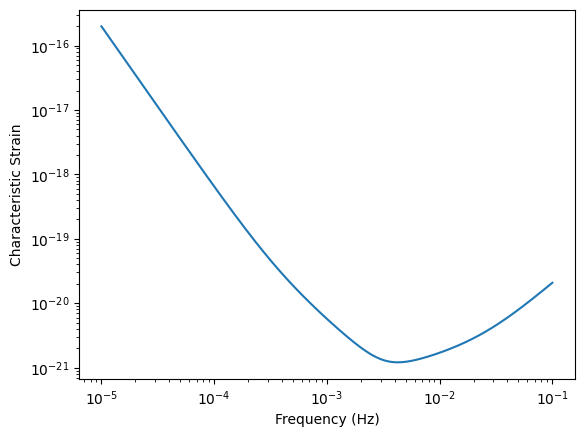
We will begin with generating the LISA sensitivity. You can do this with the lisatools.sensitivity.get_sensitivity function. Some helpful keyword arguments:
sens_fn: Type of sensitivity response function. Base sensitivity or TDI sensitivity. Base sensitivity:LISASens. TDI sensitivities are shown below.return_type: PSD, ASD, or characteristic strain.
[2]:
f = np.logspace(-5, -1, 10000)
Sn = get_sensitivity(f, sens_fn=LISASens, return_type="char_strain")
plt.loglog(f, Sn)
plt.xlabel("Frequency (Hz)")
plt.ylabel("Characteristic Strain")
[2]:
Text(0, 0.5, 'Characteristic Strain')
Stock sensitivity options can be found with lisatools.sensitivity.get_stock_sensitivity_options.
[3]:
from lisatools.sensitivity import get_stock_sensitivity_options
[4]:
get_stock_sensitivity_options()
[4]:
['X1TDISens',
 'Y1TDISens',
 'Z1TDISens',
 'XY1TDISens',
 'YZ1TDISens',
 'ZX1TDISens',
 'A1TDISens',
 'E1TDISens',
 'T1TDISens',
 'X2TDISens',
 'Y2TDISens',
 'Z2TDISens',
 'LISASens',
 'CornishLISASens',
 'FlatPSDFunction']
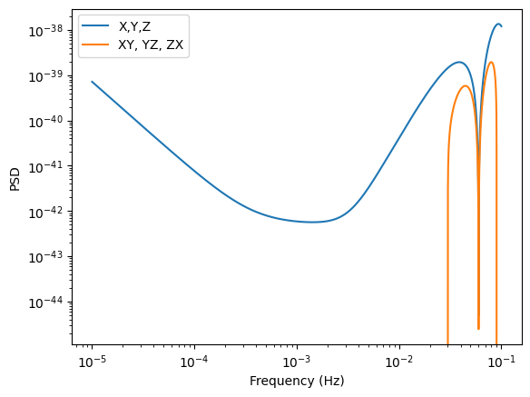
PSD for TDI channels X,Y,Z
Plot the TDI X,Y,Z channels (X1TDISens, Y1TDISens, Z1TDISens) and cross-sensitivity (XY1TDISens, YZ1TDISens, ZX1TDISens). The “1” here represents TDI generation 1. TDI 2 is available, but not the cross-terms yet. They need to be added.
[5]:
f = np.logspace(-5, -1, 10000)
Sn = get_sensitivity(f, sens_fn=X1TDISens, return_type="PSD")
plt.loglog(f, Sn, label="X,Y,Z")
Cn = get_sensitivity(f, sens_fn=XY1TDISens, return_type="PSD")
plt.loglog(f, Cn, label="XY, YZ, ZX")
plt.legend()
plt.xlabel("Frequency (Hz)")
plt.ylabel("PSD")
[5]:
Text(0, 0.5, 'PSD')
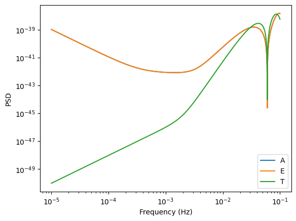
PSD for TDI channels A,E,T
Similary now for TDI A,E,T channels.
[6]:
f = np.logspace(-5, -1, 10000)
SnA = get_sensitivity(f, sens_fn=A1TDISens, return_type="PSD")
SnE = get_sensitivity(f, sens_fn=E1TDISens, return_type="PSD")
SnT = get_sensitivity(f, sens_fn=T1TDISens, return_type="PSD")
plt.loglog(f, SnA, label="A")
plt.loglog(f, SnE, label="E")
plt.loglog(f, SnT, label="T")
plt.xlabel("Frequency (Hz)")
plt.legend()
plt.ylabel("PSD")
[6]:
Text(0, 0.5, 'PSD')
Sensitivity Matrices
Sensitivity Matrices create a holder for sensitivity information across different channels. It allows for a common backend to be fed to diagnostic functions regardless if you are using AET in a length 3 array, XYZ in 3x3 matrix, or a set of basic LISASens objects. Sensitivity matrices can plot your sensitivity and update information on the fly (like if the frequency changes).
Here is a custom version of a 3x3 sensitivity matrix.
[7]:
sens_mat = SensitivityMatrix(
    f,
    [
        [X1TDISens, XY1TDISens, ZX1TDISens],
        [XY1TDISens, Y1TDISens, YZ1TDISens],
        [ZX1TDISens, YZ1TDISens, Z1TDISens],
    ],
    stochastic_params=(1.0 * YRSID_SI,),
    model=lisa_models.scirdv1,
)
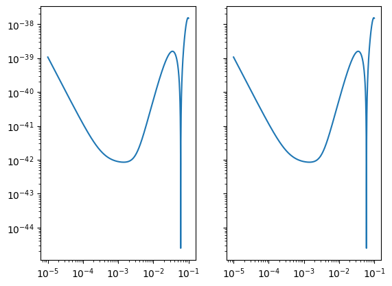
You can see the stock SensitivityMatrix options with lisatools.sensitivity.get_stock_sensitivity_matrix_options.
[8]:
from lisatools.sensitivity import get_stock_sensitivity_matrix_options
[9]:
get_stock_sensitivity_matrix_options()
[9]:
['XYZ1SensitivityMatrix', 'AET1SensitivityMatrix', 'AE1SensitivityMatrix']
[10]:
sens_mat2 = AE1SensitivityMatrix(
    f,
    # stochastic_params=None, (1.0 * YRSID_SI,),
    model=lisa_models.scirdv1,
)

sens_mat2.loglog()
[10]:
(<Figure size 640x480 with 2 Axes>, array([<Axes: >, <Axes: >], dtype=object))
You can adjust the frequencies, model, or stochastic information (see below for Stochastic) with the methods that start with “update.” For the frequency:
[11]:
sens_mat2.update_frequency_arr(np.logspace(-4, -1, 1000))
[12]:
sens_mat2.frequency_arr
[12]:
array([0.0001    , 0.00010069, 0.00010139, 0.0001021 , 0.0001028 ,
       0.00010352, 0.00010424, 0.00010496, 0.00010569, 0.00010642,
       0.00010716, 0.0001079 , 0.00010865, 0.00010941, 0.00011016,
       0.00011093, 0.0001117 , 0.00011247, 0.00011325, 0.00011404,
       0.00011483, 0.00011563, 0.00011643, 0.00011724, 0.00011805,
       0.00011887, 0.0001197 , 0.00012053, 0.00012136, 0.0001222 ,
       0.00012305, 0.00012391, 0.00012477, 0.00012563, 0.0001265 ,
       0.00012738, 0.00012826, 0.00012915, 0.00013005, 0.00013095,
       0.00013186, 0.00013278, 0.0001337 , 0.00013463, 0.00013556,
       0.0001365 , 0.00013745, 0.0001384 , 0.00013936, 0.00014033,
       0.0001413 , 0.00014228, 0.00014327, 0.00014426, 0.00014527,
       0.00014627, 0.00014729, 0.00014831, 0.00014934, 0.00015038,
       0.00015142, 0.00015247, 0.00015353, 0.00015459, 0.00015567,
       0.00015675, 0.00015783, 0.00015893, 0.00016003, 0.00016114,
       0.00016226, 0.00016339, 0.00016452, 0.00016566, 0.00016681,
       0.00016797, 0.00016913, 0.00017031, 0.00017149, 0.00017268,
       0.00017388, 0.00017508, 0.0001763 , 0.00017752, 0.00017875,
       0.00017999, 0.00018124, 0.0001825 , 0.00018377, 0.00018504,
       0.00018632, 0.00018762, 0.00018892, 0.00019023, 0.00019155,
       0.00019288, 0.00019422, 0.00019557, 0.00019692, 0.00019829,
       0.00019966, 0.00020105, 0.00020244, 0.00020385, 0.00020526,
       0.00020669, 0.00020812, 0.00020957, 0.00021102, 0.00021248,
       0.00021396, 0.00021544, 0.00021694, 0.00021844, 0.00021996,
       0.00022149, 0.00022302, 0.00022457, 0.00022613, 0.0002277 ,
       0.00022928, 0.00023087, 0.00023247, 0.00023408, 0.00023571,
       0.00023734, 0.00023899, 0.00024065, 0.00024232, 0.000244  ,
       0.00024569, 0.0002474 , 0.00024911, 0.00025084, 0.00025258,
       0.00025433, 0.0002561 , 0.00025788, 0.00025967, 0.00026147,
       0.00026328, 0.00026511, 0.00026695, 0.0002688 , 0.00027067,
       0.00027254, 0.00027443, 0.00027634, 0.00027826, 0.00028019,
       0.00028213, 0.00028409, 0.00028606, 0.00028804, 0.00029004,
       0.00029206, 0.00029408, 0.00029612, 0.00029818, 0.00030025,
       0.00030233, 0.00030443, 0.00030654, 0.00030867, 0.00031081,
       0.00031296, 0.00031514, 0.00031732, 0.00031952, 0.00032174,
       0.00032397, 0.00032622, 0.00032849, 0.00033076, 0.00033306,
       0.00033537, 0.0003377 , 0.00034004, 0.0003424 , 0.00034478,
       0.00034717, 0.00034958, 0.000352  , 0.00035445, 0.0003569 ,
       0.00035938, 0.00036187, 0.00036439, 0.00036691, 0.00036946,
       0.00037202, 0.00037461, 0.0003772 , 0.00037982, 0.00038246,
       0.00038511, 0.00038778, 0.00039047, 0.00039318, 0.00039591,
       0.00039866, 0.00040142, 0.00040421, 0.00040701, 0.00040984,
       0.00041268, 0.00041555, 0.00041843, 0.00042133, 0.00042426,
       0.0004272 , 0.00043016, 0.00043315, 0.00043615, 0.00043918,
       0.00044223, 0.0004453 , 0.00044839, 0.0004515 , 0.00045463,
       0.00045778, 0.00046096, 0.00046416, 0.00046738, 0.00047062,
       0.00047389, 0.00047718, 0.00048049, 0.00048382, 0.00048718,
       0.00049056, 0.00049396, 0.00049739, 0.00050084, 0.00050432,
       0.00050782, 0.00051134, 0.00051489, 0.00051846, 0.00052206,
       0.00052568, 0.00052933, 0.000533  , 0.0005367 , 0.00054042,
       0.00054417, 0.00054795, 0.00055175, 0.00055558, 0.00055943,
       0.00056331, 0.00056722, 0.00057116, 0.00057512, 0.00057911,
       0.00058313, 0.00058718, 0.00059125, 0.00059535, 0.00059948,
       0.00060364, 0.00060783, 0.00061205, 0.0006163 , 0.00062057,
       0.00062488, 0.00062921, 0.00063358, 0.00063798, 0.0006424 ,
       0.00064686, 0.00065135, 0.00065587, 0.00066042, 0.000665  ,
       0.00066962, 0.00067426, 0.00067894, 0.00068365, 0.0006884 ,
       0.00069317, 0.00069798, 0.00070282, 0.0007077 , 0.00071261,
       0.00071756, 0.00072253, 0.00072755, 0.0007326 , 0.00073768,
       0.0007428 , 0.00074795, 0.00075314, 0.00075837, 0.00076363,
       0.00076893, 0.00077426, 0.00077964, 0.00078505, 0.00079049,
       0.00079598, 0.0008015 , 0.00080706, 0.00081266, 0.0008183 ,
       0.00082398, 0.0008297 , 0.00083545, 0.00084125, 0.00084709,
       0.00085296, 0.00085888, 0.00086484, 0.00087084, 0.00087689,
       0.00088297, 0.0008891 , 0.00089527, 0.00090148, 0.00090773,
       0.00091403, 0.00092037, 0.00092676, 0.00093319, 0.00093966,
       0.00094618, 0.00095275, 0.00095936, 0.00096602, 0.00097272,
       0.00097947, 0.00098627, 0.00099311, 0.001     , 0.00100694,
       0.00101393, 0.00102096, 0.00102804, 0.00103518, 0.00104236,
       0.00104959, 0.00105688, 0.00106421, 0.00107159, 0.00107903,
       0.00108652, 0.00109405, 0.00110165, 0.00110929, 0.00111699,
       0.00112474, 0.00113254, 0.0011404 , 0.00114831, 0.00115628,
       0.0011643 , 0.00117238, 0.00118052, 0.00118871, 0.00119696,
       0.00120526, 0.00121362, 0.00122204, 0.00123052, 0.00123906,
       0.00124766, 0.00125632, 0.00126503, 0.00127381, 0.00128265,
       0.00129155, 0.00130051, 0.00130954, 0.00131862, 0.00132777,
       0.00133698, 0.00134626, 0.0013556 , 0.00136501, 0.00137448,
       0.00138402, 0.00139362, 0.00140329, 0.00141303, 0.00142283,
       0.0014327 , 0.00144264, 0.00145265, 0.00146273, 0.00147288,
       0.0014831 , 0.00149339, 0.00150376, 0.00151419, 0.0015247 ,
       0.00153528, 0.00154593, 0.00155665, 0.00156746, 0.00157833,
       0.00158928, 0.00160031, 0.00161141, 0.0016226 , 0.00163385,
       0.00164519, 0.00165661, 0.0016681 , 0.00167967, 0.00169133,
       0.00170307, 0.00171488, 0.00172678, 0.00173876, 0.00175083,
       0.00176298, 0.00177521, 0.00178753, 0.00179993, 0.00181242,
       0.00182499, 0.00183766, 0.00185041, 0.00186325, 0.00187617,
       0.00188919, 0.0019023 , 0.0019155 , 0.00192879, 0.00194217,
       0.00195565, 0.00196922, 0.00198288, 0.00199664, 0.0020105 ,
       0.00202445, 0.00203849, 0.00205264, 0.00206688, 0.00208122,
       0.00209566, 0.0021102 , 0.00212485, 0.00213959, 0.00215443,
       0.00216938, 0.00218444, 0.00219959, 0.00221486, 0.00223022,
       0.0022457 , 0.00226128, 0.00227697, 0.00229277, 0.00230868,
       0.0023247 , 0.00234083, 0.00235707, 0.00237342, 0.00238989,
       0.00240648, 0.00242317, 0.00243999, 0.00245692, 0.00247396,
       0.00249113, 0.00250842, 0.00252582, 0.00254335, 0.00256099,
       0.00257876, 0.00259666, 0.00261467, 0.00263282, 0.00265108,
       0.00266948, 0.002688  , 0.00270665, 0.00272543, 0.00274434,
       0.00276339, 0.00278256, 0.00280187, 0.00282131, 0.00284088,
       0.0028606 , 0.00288044, 0.00290043, 0.00292056, 0.00294082,
       0.00296123, 0.00298177, 0.00300246, 0.00302329, 0.00304427,
       0.0030654 , 0.00308666, 0.00310808, 0.00312965, 0.00315136,
       0.00317323, 0.00319525, 0.00321742, 0.00323974, 0.00326222,
       0.00328486, 0.00330765, 0.0033306 , 0.00335371, 0.00337698,
       0.00340041, 0.00342401, 0.00344776, 0.00347169, 0.00349578,
       0.00352003, 0.00354446, 0.00356905, 0.00359381, 0.00361875,
       0.00364386, 0.00366914, 0.0036946 , 0.00372024, 0.00374605,
       0.00377204, 0.00379822, 0.00382457, 0.00385111, 0.00387783,
       0.00390474, 0.00393183, 0.00395911, 0.00398658, 0.00401424,
       0.0040421 , 0.00407014, 0.00409838, 0.00412682, 0.00415546,
       0.00418429, 0.00421332, 0.00424256, 0.00427199, 0.00430164,
       0.00433148, 0.00436154, 0.0043918 , 0.00442227, 0.00445296,
       0.00448386, 0.00451497, 0.0045463 , 0.00457784, 0.0046096 ,
       0.00464159, 0.0046738 , 0.00470622, 0.00473888, 0.00477176,
       0.00480487, 0.00483821, 0.00487178, 0.00490558, 0.00493962,
       0.0049739 , 0.00500841, 0.00504316, 0.00507815, 0.00511339,
       0.00514887, 0.00518459, 0.00522057, 0.00525679, 0.00529327,
       0.00532999, 0.00536698, 0.00540422, 0.00544171, 0.00547947,
       0.00551749, 0.00555578, 0.00559433, 0.00563314, 0.00567223,
       0.00571159, 0.00575122, 0.00579112, 0.00583131, 0.00587177,
       0.00591251, 0.00595353, 0.00599484, 0.00603644, 0.00607832,
       0.0061205 , 0.00616297, 0.00620573, 0.00624879, 0.00629215,
       0.0063358 , 0.00637977, 0.00642403, 0.00646861, 0.00651349,
       0.00655869, 0.00660419, 0.00665002, 0.00669616, 0.00674262,
       0.00678941, 0.00683652, 0.00688395, 0.00693172, 0.00697981,
       0.00702824, 0.00707701, 0.00712612, 0.00717556, 0.00722535,
       0.00727548, 0.00732597, 0.0073768 , 0.00742798, 0.00747952,
       0.00753142, 0.00758368, 0.0076363 , 0.00768928, 0.00774264,
       0.00779636, 0.00785046, 0.00790493, 0.00795978, 0.00801501,
       0.00807062, 0.00812662, 0.00818301, 0.00823979, 0.00829696,
       0.00835453, 0.0084125 , 0.00847087, 0.00852964, 0.00858883,
       0.00864842, 0.00870843, 0.00876886, 0.0088297 , 0.00889097,
       0.00895266, 0.00901478, 0.00907733, 0.00914031, 0.00920373,
       0.00926759, 0.0093319 , 0.00939665, 0.00946185, 0.0095275 ,
       0.00959361, 0.00966017, 0.0097272 , 0.0097947 , 0.00986266,
       0.00993109, 0.01      , 0.01006939, 0.01013925, 0.01020961,
       0.01028045, 0.01035178, 0.01042361, 0.01049593, 0.01056876,
       0.01064209, 0.01071593, 0.01079029, 0.01086516, 0.01094055,
       0.01101646, 0.0110929 , 0.01116987, 0.01124737, 0.01132541,
       0.011404  , 0.01148312, 0.0115628 , 0.01164303, 0.01172382,
       0.01180517, 0.01188708, 0.01196956, 0.01205261, 0.01213624,
       0.01222045, 0.01230524, 0.01239062, 0.0124766 , 0.01256317,
       0.01265034, 0.01273811, 0.0128265 , 0.0129155 , 0.01300511,
       0.01309535, 0.01318621, 0.01327771, 0.01336984, 0.01346261,
       0.01355602, 0.01365008, 0.01374479, 0.01384016, 0.01393619,
       0.01403289, 0.01413026, 0.0142283 , 0.01432703, 0.01442644,
       0.01452654, 0.01462733, 0.01472883, 0.01483103, 0.01493393,
       0.01503755, 0.01514189, 0.01524696, 0.01535275, 0.01545928,
       0.01556654, 0.01567455, 0.01578331, 0.01589283, 0.0160031 ,
       0.01611414, 0.01622595, 0.01633854, 0.01645191, 0.01656606,
       0.01668101, 0.01679675, 0.0169133 , 0.01703065, 0.01714882,
       0.01726781, 0.01738762, 0.01750827, 0.01762975, 0.01775208,
       0.01787526, 0.01799929, 0.01812418, 0.01824993, 0.01837656,
       0.01850407, 0.01863246, 0.01876175, 0.01889193, 0.01902301,
       0.01915501, 0.01928792, 0.01942175, 0.01955651, 0.0196922 ,
       0.01982884, 0.01996642, 0.02010496, 0.02024447, 0.02038493,
       0.02052638, 0.0206688 , 0.02081222, 0.02095662, 0.02110203,
       0.02124845, 0.02139589, 0.02154435, 0.02169384, 0.02184436,
       0.02199593, 0.02214855, 0.02230223, 0.02245698, 0.0226128 ,
       0.0227697 , 0.02292769, 0.02308678, 0.02324697, 0.02340827,
       0.02357069, 0.02373424, 0.02389893, 0.02406475, 0.02423173,
       0.02439986, 0.02456916, 0.02473964, 0.0249113 , 0.02508415,
       0.0252582 , 0.02543346, 0.02560993, 0.02578763, 0.02596656,
       0.02614673, 0.02632815, 0.02651084, 0.02669478, 0.02688001,
       0.02706652, 0.02725433, 0.02744343, 0.02763385, 0.02782559,
       0.02801867, 0.02821308, 0.02840884, 0.02860596, 0.02880444,
       0.0290043 , 0.02920556, 0.0294082 , 0.02961225, 0.02981772,
       0.03002462, 0.03023295, 0.03044272, 0.03065395, 0.03086665,
       0.03108082, 0.03129648, 0.03151363, 0.0317323 , 0.03195248,
       0.03217418, 0.03239743, 0.03262222, 0.03284857, 0.0330765 ,
       0.033306  , 0.0335371 , 0.0337698 , 0.03400412, 0.03424006,
       0.03447764, 0.03471687, 0.03495776, 0.03520031, 0.03544456,
       0.03569049, 0.03593814, 0.0361875 , 0.03643859, 0.03669142,
       0.03694601, 0.03720237, 0.0374605 , 0.03772042, 0.03798215,
       0.0382457 , 0.03851107, 0.03877828, 0.03904735, 0.03931829,
       0.0395911 , 0.03986581, 0.04014242, 0.04042096, 0.04070142,
       0.04098384, 0.04126821, 0.04155455, 0.04184289, 0.04213322,
       0.04242556, 0.04271994, 0.04301636, 0.04331483, 0.04361538,
       0.04391801, 0.04422274, 0.04452959, 0.04483856, 0.04514968,
       0.04546295, 0.04577841, 0.04609604, 0.04641589, 0.04673795,
       0.04706225, 0.0473888 , 0.04771761, 0.0480487 , 0.0483821 ,
       0.0487178 , 0.04905584, 0.04939622, 0.04973896, 0.05008408,
       0.05043159, 0.05078152, 0.05113388, 0.05148867, 0.05184594,
       0.05220568, 0.05256791, 0.05293266, 0.05329994, 0.05366977,
       0.05404216, 0.05441714, 0.05479472, 0.05517492, 0.05555776,
       0.05594326, 0.05633143, 0.05672229, 0.05711586, 0.05751217,
       0.05791123, 0.05831305, 0.05871766, 0.05912508, 0.05953533,
       0.05994843, 0.06036439, 0.06078323, 0.06120498, 0.06162966,
       0.06205729, 0.06248788, 0.06292146, 0.06335805, 0.06379767,
       0.06424034, 0.06468608, 0.06513491, 0.06558686, 0.06604194,
       0.06650018, 0.0669616 , 0.06742622, 0.06789407, 0.06836516,
       0.06883952, 0.06931717, 0.06979814, 0.07028244, 0.07077011,
       0.07126115, 0.07175561, 0.07225349, 0.07275484, 0.07325965,
       0.07376798, 0.07427982, 0.07479523, 0.0753142 , 0.07583678,
       0.07636298, 0.07689284, 0.07742637, 0.0779636 , 0.07850456,
       0.07904928, 0.07959777, 0.08015007, 0.0807062 , 0.08126619,
       0.08183007, 0.08239786, 0.08296959, 0.08354528, 0.08412497,
       0.08470868, 0.08529644, 0.08588829, 0.08648423, 0.08708431,
       0.08768856, 0.088297  , 0.08890966, 0.08952657, 0.09014776,
       0.09077327, 0.09140311, 0.09203732, 0.09267593, 0.09331898,
       0.09396648, 0.09461848, 0.095275  , 0.09593608, 0.09660175,
       0.09727203, 0.09794697, 0.09862658, 0.09931092, 0.1       ])
Orbits
Orbital information is read in from files and stored in an Orbits class. There are two stock options: EqualArmlengthOrbits and ESAOrbits. The files for the classes are directly from the LISAOrbits code. The lisatools Orbits class can take any file that is output from the LISAOrbits code.
Each orbit class, after instantiation, must be configured. This transforms the input file values into the setup used for analysis. During configuration, you can pass a time array, timestep, or you can ask the orbit class to setup for linear interpolation by passing linear_interp_setup=True. This setup will add enough points to the time array to make linear interpolation accurate enough.
[13]:
equal = EqualArmlengthOrbits()
equal.configure(linear_interp_setup=True)

esa = ESAOrbits()
esa.configure(linear_interp_setup=True)
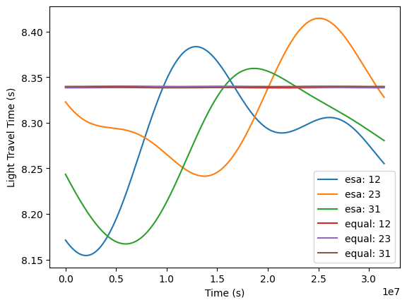
You can access various information on the orbits with the methods that begin with get. You can get light travel times, spacecraft positions, or link normal vectors. These functions require a linear interpolation setup.
Link light travel times.
[14]:
t_vals = np.linspace(0.0, np.min([esa.t_base.max(), equal.t_base.max()]), 1000)
for orbits, name in zip([esa, equal], ["esa", "equal"]):
    for link in [12, 23, 31]:
        plt.plot(t_vals, orbits.get_light_travel_times(t_vals, link), label=f"{name}: {link}")
plt.legend()
plt.ylabel("Light Travel Time (s)")
plt.xlabel("Time (s)")
[14]:
Text(0.5, 0, 'Time (s)')
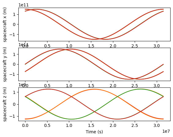
Spacecraft positions
[15]:
t_vals = np.linspace(0.0, np.min([esa.t_base.max(), equal.t_base.max()]), 1000)
fig, ax = plt.subplots(3, 1)
for orbits, name in zip([esa, equal], ["esa", "equal"]):
    for sc in [1, 2, 3]:
        pos = orbits.get_pos(t_vals, sc)
        for i in range(3):
            ax[i].plot(t_vals, pos[:, i], color=f"C{sc}", label=f"{name}: {link}")
ax[0].set_ylabel("spacecraft x (m)")
ax[1].set_ylabel("spacecraft y (m)")
ax[2].set_ylabel("spacecraft z (m)")
ax[2].set_xlabel("Time (s)")
[15]:
Text(0.5, 0, 'Time (s)')
Defining a LISAModel
A LISAModel is a combination of sensitivity information and orbits. For the sensitivity, we define a two parameter model based on the OMS noise and acceleration noise.
[16]:
oms_noise_term = (13.0e-12) ** 2
acceleration_noise_term = (2.0e-15) ** 2
new_lisa = LISAModel(oms_noise_term, acceleration_noise_term, equal, "new_lisa")
[17]:
# example stock model
get_available_default_lisa_models()
[17]:
[LISAModel(Soms_d=2.25e-22, Sa_a=9e-30, orbits=<lisatools.detector.DefaultOrbits object at 0x128f126c0>, name='scirdv1'),
 LISAModel(Soms_d=9.999999999999999e-23, Sa_a=9e-30, orbits=<lisatools.detector.DefaultOrbits object at 0x12fc18560>, name='proposal'),
 LISAModel(Soms_d=9.999999999999999e-23, Sa_a=5.76e-30, orbits=<lisatools.detector.DefaultOrbits object at 0x118aa04a0>, name='mrdv1'),
 LISAModel(Soms_d=6.241e-23, Sa_a=5.76e-30, orbits=<lisatools.detector.DefaultOrbits object at 0x11870f470>, name='sangria')]
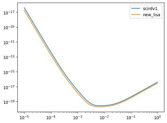
Compare two models.
[18]:
f = np.logspace(-5, 0, 10000)

for model in [scirdv1, new_lisa]:
    Sn = get_sensitivity(f, sens_fn="LISASens", model=model)
    plt.loglog(f, Sn, label=model.name)
plt.legend()
[18]:
<matplotlib.legend.Legend at 0x148514620>
Diagnostics
LISA Analysis Tools comes with a wide variety of diagnostic computations. These can be used in actual pipelines. However, they are slower, so these should mainly be used to check faster Likelihood methods.
To begin, we will define a basic sine wave as our waveform.
[19]:
def sine_waveform(A, f0, phi0, t_arr):
    return A * np.sin(2 * np.pi * f0 * t_arr + phi0)
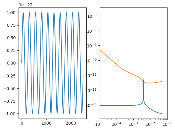
Inner Product
You can take the inner product between to waveforms. See the inner product documentation for keyword arguments and details.
[20]:
# create some fake signals first

A = 1e-22
f0 = 4e-3
phi0 = 0.2

dt = 10.0
t_arr = np.arange(0.0, YRSID_SI, dt)
df = 1 / (len(t_arr) * dt)
h1 = sine_waveform(A, f0, 0.0, t_arr)
h2 = sine_waveform(A, f0, phi0, t_arr)

fig, (ax1, ax2) = plt.subplots(1, 2)
ax1.plot(t_arr[:250], h1[:250])

freqs = np.fft.rfftfreq(len(h1), dt)
ax2.loglog(freqs, np.abs(np.fft.rfft(h1)))

ax2.loglog(freqs, (get_sensitivity(freqs, sens_fn="LISASens", model="sangria", stochastic_params=(YRSID_SI,)) / (4 * df)) ** (1/2))

val = inner_product(h1, h2, dt=dt, psd="LISASens", psd_kwargs=dict(model="sangria", stochastic_params=(YRSID_SI,)))
print(f"Inner product <h1|h2>: {val}")

complex_val = inner_product(h1, h2, dt=dt, psd="LISASens", psd_kwargs=dict(model="sangria", stochastic_params=(YRSID_SI,)), complex=True)
print(f"Complex inner product <h1|h2>: {complex_val}, phase maximized value: {np.abs(complex_val)}")

normalized_val = inner_product(h1, h2, dt=dt, psd="LISASens", psd_kwargs=dict(model="sangria", stochastic_params=(YRSID_SI,)), normalize=True)
print(f"Normalized inner product <h1|h2>: {normalized_val}")

ax2.set_xlim(1e-5,)
/Users/mlkatz1/anaconda3/envs/lisa_env/lib/python3.12/site-packages/lisatools/detector.py:633: RuntimeWarning: divide by zero encountered in divide
  Sa_a = Sa_a_in * (1.0 + (0.4e-3 / frq) ** 2) * (1.0 + (frq / 8e-3) ** 4)
/Users/mlkatz1/anaconda3/envs/lisa_env/lib/python3.12/site-packages/lisatools/detector.py:635: RuntimeWarning: divide by zero encountered in power
  Sa_d = Sa_a * (2.0 * np.pi * frq) ** (-4.0)
/Users/mlkatz1/anaconda3/envs/lisa_env/lib/python3.12/site-packages/lisatools/detector.py:637: RuntimeWarning: invalid value encountered in multiply
  Sa_nu = Sa_d * (2.0 * np.pi * frq / C_SI) ** 2
/Users/mlkatz1/anaconda3/envs/lisa_env/lib/python3.12/site-packages/lisatools/detector.py:642: RuntimeWarning: divide by zero encountered in divide
  Soms_d = Soms_d_in * (1.0 + (2.0e-3 / f) ** 4)
/Users/mlkatz1/anaconda3/envs/lisa_env/lib/python3.12/site-packages/lisatools/detector.py:644: RuntimeWarning: invalid value encountered in multiply
  Soms_nu = Soms_d * (2.0 * np.pi * frq / C_SI) ** 2
/Users/mlkatz1/anaconda3/envs/lisa_env/lib/python3.12/site-packages/lisatools/stochastic.py:178: RuntimeWarning: divide by zero encountered in power
  * (f ** (-7.0 / 3.0))
Inner product <h1|h2>: 1981.3392667268324
Complex inner product <h1|h2>: (1981.3392667268322+401.63841799838985j), phase maximized value: 2021.6376304090381
Normalized inner product <h1|h2>: 0.9800664328144687
[20]:
(1e-05, np.float64(0.10206431774793984))
SNR
[21]:
opt_snr = snr(h1, dt=dt, psd="LISASens", psd_kwargs=dict(model="sangria", stochastic_params=(YRSID_SI,)))
print(f"Optimal SNR <h1|h1>^(1/2): {opt_snr}")

det_snr = snr(h1, data=h2, dt=dt, psd="LISASens", psd_kwargs=dict(model="sangria", stochastic_params=(YRSID_SI,)))
print(f"Detected SNR against data h1 <h1|h2> / <h1|h1>^(1/2): {det_snr}")
Optimal SNR <h1|h1>^(1/2): 44.96261510900951
Detected SNR against data h1 <h1|h2> / <h1|h1>^(1/2): 44.06637073762678
Perturbed Waveform
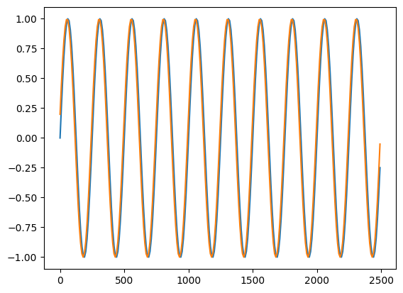
Get a waveform with a small perturbation to a parameter.
[22]:
# set quantities for below calculations
params = np.array([np.log(A), f0 * 1e3, phi0])
eps = 1e-9
index = 1

parameter_transforms = {
    0: np.exp,
    1: lambda x: x / 1e3
}

transform_fn = TransformContainer(parameter_transforms=parameter_transforms)
[23]:
params = np.array([np.log(A), f0 * 1e3, phi0])
step = 1e-9
index = 1

parameter_transforms = {
    0: np.exp,
    1: lambda x: x / 1e3
}

transform_fn = TransformContainer(parameter_transforms=parameter_transforms)

# will return 2D
dh = h_var_p_eps(
    step,
    sine_waveform,
    params,
    index,
    waveform_args=(t_arr,),
    parameter_transforms=transform_fn
)

plt.plot(t_arr[:250], h1[:250] / np.abs(h1[:250]).max())
plt.plot(t_arr[:250], dh[0, :250] / np.abs(dh[0, :250]).max())
[23]:
[<matplotlib.lines.Line2D at 0x148caf8f0>]
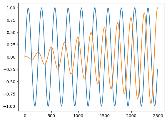
Derivative of Waveform
Compute the derivative of a waveform with respect to a parameter.
[24]:
dhdlam = dh_dlambda(
    eps,
    sine_waveform,
    params,
    index,
    waveform_args=(t_arr,),
    parameter_transforms=transform_fn
)

# TODO: check this?
plt.plot(t_arr[:250], h1[:250] / np.abs(h1[:250]).max())
plt.plot(t_arr[:250], dhdlam[0, :250] / np.abs(dhdlam[0, :250]).max())
[24]:
[<matplotlib.lines.Line2D at 0x148d8d040>]
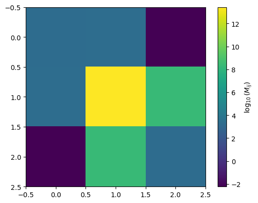
Information Matrix and Covariance
Information matrix and covariance matrices.
[25]:
params = np.array([np.log(A), f0 * 1e3, phi0])
eps = 1e-9

info_mat_args = (eps, sine_waveform, params)
info_mat_kwargs = dict(
    deriv_inds=None,
    inner_product_kwargs={
        "psd": "LISASens",
        "psd_kwargs": dict(model="sangria", stochastic_params=(YRSID_SI,)),
        "dt": dt,
    },
    return_derivs=False,
    waveform_args=(t_arr,),
    parameter_transforms=transform_fn,
)
im = info_matrix(*info_mat_args, **info_mat_kwargs)

cov = covariance(
    *info_mat_args,
    info_mat=None,
    diagonalize=False,
    return_info_mat=False,
    precision=True,
    **info_mat_kwargs,
)
print(cov)
[[ 4.94652789e-04 -1.34367659e-13  1.19036834e-08]
 [-1.34367659e-13  1.46157988e-13 -1.45604730e-08]
 [ 1.19036834e-08 -1.45604730e-08  1.95551222e-03]]
Visualizing your information matrix.
[26]:
plt.imshow(np.log10(im))
plt.colorbar(label=r"$\log_{10}(M_{ij})$")
[26]:
<matplotlib.colorbar.Colorbar at 0x14fe7e480>
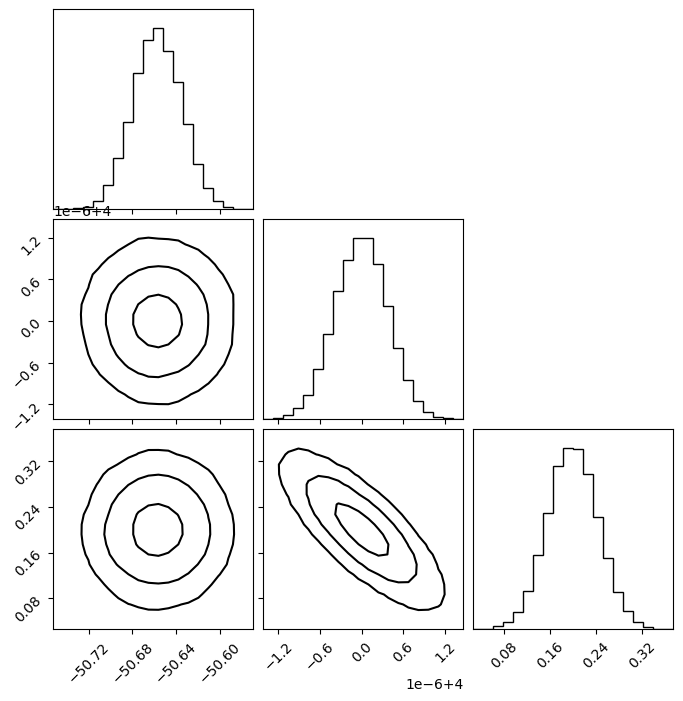
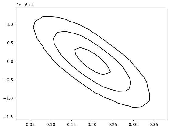
Plot Covariance in Corner Plot
You can plot a corner plot by generated samples from the covariance matrix.s
[27]:
plot_kwargs = dict(
    plot_density=False,
    plot_datapoints=False,  # fake in this case
    smooth=0.8,
    levels=1 - np.exp(-0.5 * np.array([1, 2, 3]) ** 2)  # 1, 2, 3 sigma
)

plot_covariance_corner(
    params,
    cov,
    **plot_kwargs
)
[27]:

Make a single contour plot.
[28]:
fig, ax = plt.subplots(1,1)

plot_covariance_contour(
    params,
    cov,
    2,
    1,
    ax=ax,
    **plot_kwargs
)
[28]:
<Axes: >
Get Eigeninfo of a matrix (high-precision capability)
Get eigenvectors and eigenvalues of a matrix with high-precision capability.
[29]:
evals, evecs = get_eigeninfo(
    cov, high_precision=False
)
evals, evecs
[29]:
(array([4.94652788e-04, 1.95551222e-03, 3.77427245e-14]),
 array([[ 1.00000000e+00,  8.14841119e-06,  9.24577470e-11],
        [-3.17858065e-11, -7.44586141e-06,  1.00000000e+00],
        [-8.14841119e-06,  1.00000000e+00,  7.44586140e-06]]))
Scale to a given SNR
Scaled an injection signal to a given SNR in place.
[30]:
target_snr = 30.0

# with 0.0 for the phase here, h1/h1_scaled will have a nan at the beginning.
h1 = sine_waveform(A, f0, 0.2, t_arr)

h1_scaled = scale_to_snr(
    target_snr,
    h1,
    dt=dt,
    psd="LISASens",
    psd_kwargs=dict(model="sangria", stochastic_params=(YRSID_SI,))
)

print(h1 / h1_scaled)
[1.49875455 1.49875455 1.49875455 ... 1.49875455 1.49875455 1.49875455]
/Users/mlkatz1/anaconda3/envs/lisa_env/lib/python3.12/site-packages/lisatools/detector.py:633: RuntimeWarning: divide by zero encountered in divide
  Sa_a = Sa_a_in * (1.0 + (0.4e-3 / frq) ** 2) * (1.0 + (frq / 8e-3) ** 4)
/Users/mlkatz1/anaconda3/envs/lisa_env/lib/python3.12/site-packages/lisatools/detector.py:635: RuntimeWarning: divide by zero encountered in power
  Sa_d = Sa_a * (2.0 * np.pi * frq) ** (-4.0)
/Users/mlkatz1/anaconda3/envs/lisa_env/lib/python3.12/site-packages/lisatools/detector.py:637: RuntimeWarning: invalid value encountered in multiply
  Sa_nu = Sa_d * (2.0 * np.pi * frq / C_SI) ** 2
/Users/mlkatz1/anaconda3/envs/lisa_env/lib/python3.12/site-packages/lisatools/detector.py:642: RuntimeWarning: divide by zero encountered in divide
  Soms_d = Soms_d_in * (1.0 + (2.0e-3 / f) ** 4)
/Users/mlkatz1/anaconda3/envs/lisa_env/lib/python3.12/site-packages/lisatools/detector.py:644: RuntimeWarning: invalid value encountered in multiply
  Soms_nu = Soms_d * (2.0 * np.pi * frq / C_SI) ** 2
/Users/mlkatz1/anaconda3/envs/lisa_env/lib/python3.12/site-packages/lisatools/stochastic.py:178: RuntimeWarning: divide by zero encountered in power
  * (f ** (-7.0 / 3.0))
Bias estimate
Approximate waveform with a purposeful bias on the amplitude. Use the C-V bias estimate using our underlying covariance methods.
[31]:
def sine_waveform_approx(A, f0, phi0, t_arr):
    return A * 1.03 * np.sin(2 * np.pi * (f0 * 0.98) * t_arr + phi0)
[32]:
sys_err, bias = cutler_vallisneri_bias(
    sine_waveform,
    sine_waveform_approx,
    params,
    eps,
    parameter_transforms=transform_fn,
    inner_product_kwargs={
        "psd": "LISASens",
        "psd_kwargs": dict(model="sangria", stochastic_params=(YRSID_SI,)),
        "dt": dt,
    },
    waveform_true_args=(t_arr,),
    waveform_approx_args=(t_arr,),
)
print(sys_err, bias)
[2.02172681e+03 1.59046154e+04 1.94227122e-01] [ 1.00005281e+00 -7.75106867e-10 1.72300784e-04]
Data / Residual / Signal Container
This container is a holder for data, residuals, or templates. These communicate with other classes like the Sensitivity Matrix to streamline different analyses.
[33]:
from lisatools.datacontainer import DataResidualArray
[34]:
arr1 = sine_waveform(A, f0, phi0, t_arr)
arr2 = sine_waveform(A, f0, phi0 + np.pi / 2, t_arr)

data = DataResidualArray([arr1, arr2], dt=dt)
[35]:
data.loglog(char_strain=True)
[35]:
(<Figure size 640x480 with 2 Axes>, array([<Axes: >, <Axes: >], dtype=object))
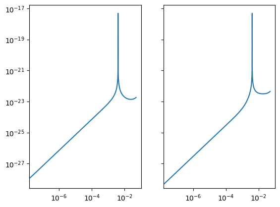
Analysis Container
The AnalysisContainer brings together the SensitivityMatrix and the DataResidualArray to perform a variety of computations.
[36]:
from lisatools.analysiscontainer import AnalysisContainer
from lisatools.sensitivity import LISASens

sens_mat = SensitivityMatrix(data.f_arr, [LISASens, LISASens], stochastic_params=(YRSID_SI,))
analysis = AnalysisContainer(data, sens_mat)
[37]:
analysis.loglog()
/Users/mlkatz1/anaconda3/envs/lisa_env/lib/python3.12/site-packages/lisatools/sensitivity.py:747: RuntimeWarning: invalid value encountered in multiply
  plot_in = np.sqrt(self.frequency_arr * plot_in)
[37]:
(<Figure size 640x480 with 2 Axes>, array([<Axes: >, <Axes: >], dtype=object))
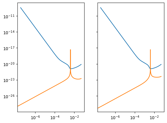
Direct computations on the residual contained in the DataResidualArrray.
[38]:
analysis.inner_product()
[38]:
1646.1603122108786
[39]:
analysis.likelihood()
[39]:
np.float64(-inf)
[40]:
analysis.likelihood(source_only=True)
[40]:
-823.0801561054393
[41]:
analysis.likelihood(noise_only=True)
[41]:
np.float64(-inf)
[42]:
analysis.snr()
[42]:
40.57290120524879
Build a template and then compare it to the data.
[43]:
# build template
h_test = DataResidualArray([
    sine_waveform(A * 1.05, f0, phi0 + 0.002, t_arr),
    sine_waveform(A * 1.05, f0, phi0 + 0.002 + np.pi / 2., t_arr)
] , dt=dt)

print(f"Template Inner product: {analysis.template_inner_product(h_test)}") # , analysis.template_likelihood, analysis.template_snr
print(f"Template SNR: {analysis.template_snr(h_test)}") # , analysis.template_likelihood, analysis.template_snr
print(f"Template Likelihood: {analysis.template_likelihood(h_test)}") # , analysis.template_likelihood, analysis.template_snr
Template Inner product: 1728.4648708859095
Template SNR: (np.float64(42.60154626551122), np.float64(40.572820059473216))
Template Likelihood: -2.0611573257758664
Build a template generation model and add to the AnalysisContainer
This allows for inputing parameters and waveform settings directly to the AnalysisContainer for computations.
[44]:
def signal_model_sine(A, f0, phi0, t_arr):
    template = DataResidualArray([
        sine_waveform(A, f0, phi0, t_arr),
        sine_waveform(A, f0, phi0 + np.pi / 2., t_arr)
    ] , dt=dt)
    return template

analysis.signal_gen = signal_model_sine
[45]:
print(f"With parameters likelihood: {analysis.calculate_signal_likelihood(A, f0, phi0, t_arr, source_only=True)}")
print(f"With parameters snr: {analysis.calculate_signal_snr(A, f0, phi0, t_arr)}")
print(f"With parameters inner product: {analysis.calculate_signal_inner_product(A, f0, phi0, t_arr)}")

print("Adjust amplitude:")
print(f"With parameters likelihood: {analysis.calculate_signal_likelihood(A * 1.03, f0, phi0, t_arr, source_only=True)}")
print(f"With parameters snr: {analysis.calculate_signal_snr(A * 1.03, f0, phi0, t_arr)}")
print(f"With parameters inner product: {analysis.calculate_signal_inner_product(A * 1.03, f0, phi0, t_arr)}")
With parameters likelihood: -0.0
With parameters snr: (np.float64(40.57290120524879), np.float64(40.57290120524879))
With parameters inner product: 1646.1603122108786
Adjust amplitude:
With parameters likelihood: -0.7407721404947551
With parameters snr: (np.float64(41.79008824140625), np.float64(40.57290120524879))
With parameters inner product: 1695.545121577205
Comparing XYZ and AET
The XYZ TDI channels have correlated noise. In matrix form, you can imagine this as
.
For AET, this becomes diagonalized:
In the inner product equation, the multiplication of the template and noise is given as \((\mathbf{h}^T \mathbf{C}^{-1} \mathbf{h})\). In the XYZ basis, the full 3x3 matrix at each frequency must be inverted. In the AET basis, the inversion is equivalent to taking 1 over the sensitivity value themselves.
A good check is to verify that your inner product values are equivalent in both bases. To do this, you need real TDI templates. So, we will use GBGPU to put in one Galactic binary waveform.
[46]:
# setup a data stream
dt = 10.0
Tobs = YRSID_SI / 2.0
N = int(Tobs / dt)
Tobs = N * dt
t = np.arange(N) * dt

data_xyz = DataResidualArray(
    [
        np.zeros_like(t),
        np.zeros_like(t),
        np.zeros_like(t),
    ],
    dt=dt,
)

data_aet = DataResidualArray(
    [
        np.zeros_like(t),
        np.zeros_like(t),
        np.zeros_like(t),
    ],
    dt=dt,
)

# build waveforms
from gbgpu.gbgpu import GBGPU
gb = GBGPU()
gb.run_wave(
    1e-23, 0.003, 1e-17, 0.0, 0.4, 0.8, 0.9, 0.3, 0.5, T=Tobs, dt=dt, oversample=4
)

# inject waveforms
data_xyz[:, gb.start_inds[0] : gb.start_inds[0] + gb.A.shape[-1]] = (
    gb.XYZf[:]
)
data_aet[:, gb.start_inds[0] : gb.start_inds[0] + gb.A.shape[-1]] = (
    np.asarray(AET(*gb.XYZf[0]))
)

# set sensitivity matrices
sens_xyz = XYZ1SensitivityMatrix(data_xyz.f_arr, model="scirdv1")
sens_aet = AET1SensitivityMatrix(data_aet.f_arr, model="scirdv1")

ac_xyz = AnalysisContainer(data_xyz, sens_xyz)
ac_aet = AnalysisContainer(data_aet, sens_aet)

print(ac_xyz.inner_product(), ac_aet.inner_product())
print(ac_xyz.likelihood(source_only=True), ac_aet.likelihood(source_only=True))

# TODO: currently a small difference in noise-included likelihoodm
print(ac_xyz.likelihood(), ac_aet.likelihood())
19.134165338394837 19.134165338394727
-9.567082669197418 -9.567082669197363
108203542.2031658 108203940.3557624