Convolutional Neural Network for Gravitational Wave Analysis

Abstract:

For my final project in EECS 349 (Northwestern University), I investigated the use of neural networks, specifically convolutional neural networks, in gravitational wave data analysis related to the Laser Interferometer Space Antenna (LISA). I worked on this project by myself. My contact email address is mikekatz04@gmail.com.

LISA is a future space-based mission to measure gravitational waves created by the most extreme objects in the universe: black holes, neutron stars, and white dwarf stars. While the mission is underway, the detector will be detecting upwards of 10000+ gravitational wave sources simultaneously in a singular data stream. One of the main sources of interest are Extreme Mass Ratio Inspirals (EMRIs). EMRIs occur when a small black hole, like those resulting from dying stars, orbit at close to the speed of light around massive black holes existing in the centers of galaxies. The mass ratio between the black holes is usually 10000 or more. These orbits are very complex, and are still not well understood theoretically or computationally. These sources will help shed light on extreme dynamical systems in the centers of galaxies, as well as help refine our understanding of the General Theory of Relativity. The state of data analysis for EMRIs is wide open. I wanted to begin to investigate using machine learning to help us accomplish many sorts of difficult data-related tasks.

For this project, I focused on the amplitude of the Fourier transform of an EMRI gravitational wave time series. The amplitudes from all frequency bins became the features used here. Two tasks were of most interest to me for this project. The first task was to use regression to predict the three fundamental frequencies that make up the complex time-domain EMRI signal. To do this, I used a 1-dimensional convolutional neural network with the amplitudes in each frequency bin as the features and the theoretically determined fundamental frequencies as the labels. I additionally used a nearest neighbors algorithm for comparison. However, the goal was to make a scalable project that can query fast with the data after many input waveforms. A nearest neighbors regressor is not expected to scale well in terms of query time, and, therefore, was not the main focus of the project.

The second aspect of the project was to use a convolutional autoencoder to reduce the dimensionality of the amplitude spectrum from 800 bins to a lower dimensionality. This is for the purpose of using future regression studies with techniques such as gaussian process regression. For this task, the features were the same as above, but the labels were the features themselves, as in any autoencoder. Below are two images showing the output of the autoencoder compared to the initial amplitudes.

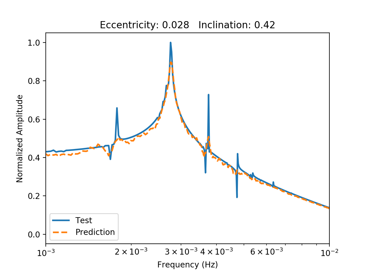
The amplitude spectrum is shown above for a binary with low eccentricity (0.028) and a lower inclination (0.42 radians). The prediction from the autoencoder is shown in dotted orange.

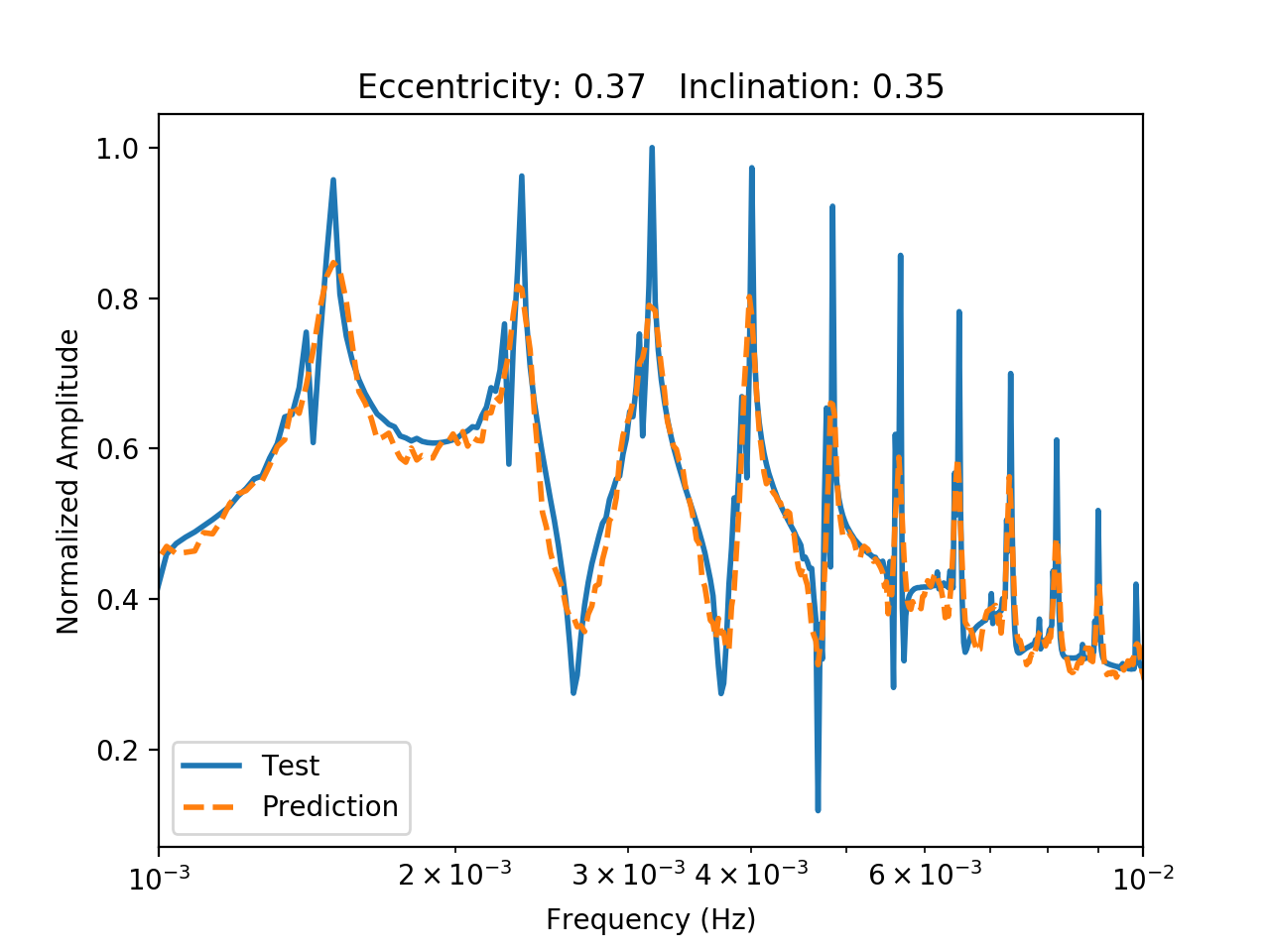
The amplitude spectrum is shown above for a binary with a higher eccentricity (0.37) and a lower inclination (0.35 radians). The prediction from the autoencoder is shown in dotted orange. Higher eccentricities lead to signals with higher order harmonics.

My key findings for the fundamental frequency regressor were that reducing the kernel size, increasing the number of convolutional layers, or changing the output layer activation function from linear to ReLu improves the accuracy and precision of the fit. Most of the CNNs outperformed the nearest neighbors regressor. For the autoencoder, more convolutional layers performed worse. The ideal layers for autencoding was found to be two convolutional layers for encoding and 3 for decoding.

Data Creation

For this project, I generated datasets using a waveform generator by Chua et al 2017. I used the Numerical Kludge (NK) waveform, which is fast compared to high fidelity waveforms, but slow compared to analytical generators. I fixed all of the parameters of the waveform generator except for the eccentricity and inclination. The eccentricity defines the ellipticity of the orbit away from circularity. The inclination represents the angle of the orbital plane away from the equatorial axis of the large black hole. I sampled 12 hrs of waveform data on a grid of eccentricities from 0.01 to 0.4 and inclinations from 0.01 to 0.79 radians. My training set consisted of 10000 of these waveforms. I then used numpy’s discrete Fourier transform (DFT) to find the amplitude spectrum of each waveform. True EMRI signals vary from 0.1 mHz to 100 mHz, even though the DFT varies from 0.001 mHz to 1 Hz. Therefore, I cut down the dataset from 21601 frequency bins to the 859 bins within those two limiting frequencies. I then normalized the amplitude spectrum so the convolutional network could focus on the shape of each waveform rather than the overall magnitude. This is because extrinsic quantities like the distance can modulate the signal amplitude; I wanted this initial trainer to focus on the intrinsic quantities specific to each system.

In addition to the amplitude spectrum, I also had the generator output the trajectory of the orbit so that I knew the eccentricity and inclination. With these values in hand, I was able to find the theoretical fundamental frequencies of the orbit which are determined from orbital parameters. These values became the labels attached to each amplitude spectrum. At training time, I rescaled the ranges of the three fundamental frequency from zero to one.

Due to the computation time for generating these waveforms, I decided to generate a smaller test set than I plan to use in the future. Within the eccentricity and inclination limits stated above, I drew each quantity from a uniform distribution on each parameter to generate 100 test waveforms. Once again, I found the fundamental frequencies of the orbit in the same way as mentioned above.

Fundamental Frequency Regressor (FFR)

FFR Methods

One issue with Fourier transforms is spectral leakage between neighboring bins. This makes finding true peaks an issue. Additionally, the bins are not centered on the integer multiples of the fundamental frequencies (higher order harmonics); therefore, locating peaks can only help determine these integer multiples of the fundamental modes to a degree of certainty equal to the bin width. Also, more peaks helps further determine the system of equations we could algebraically use to determine the frequencies. However, lower eccentricity signals radiate at a small amount of frequencies, making the system of equations impossible to solve.

Machine learning can be used to learn the shapes of amplitude spectral peaks and relate them to actual fundamental frequency values, allowing for a regressor that can handle spectral leakage and a small amount of peaks. For this, it was clear I needed to use a convolutional neural network that could understand the shape of the 1D spectrum, associating neighboring features to understand where peaks are and how to match them to the three fundamental modes. I tried many different architectures of the convolutional network to see which would be the best for this initial investigation. I did not use cross-validation due to computation time and the fact that my training set was gridded, which is similar to what would be done in reality. However, this would be an interesting investigation to locate which areas of the parameter space are more sensitive to less waveforms (see Future Work).

For all models I tried, I used 2 or 4 convolutional layers (CL), each with a corresponding max pooling layer with size 2 pooling. These all had ReLu activation functions. I also tried different kernel sizes (K) at 10 or 50. For the initial convolutional layer, I used 32 filters. After this, each convolutional layer had 64 filters. After the final max pooling layer, the tensor was flattened and then fed into a dense layer with 1024 neurons with ReLu activation. After this dense layer, I had a dropout layer to remove 40 percent of the previous layer’s neurons. The output layer had 3 neurons, one for each fundamental frequency, with a linear activation (Act) for regression. For one model, I used ReLu activation on the output layer since the frequencies are positive definite. The loss function I used was the mean squared error. Each model was trained for 200 epochs. All of my CNN models were designed using Keras with a Tensorflow backend. Below are the learning curves for the model with a kernel size of 50, ReLu output layer activation, and two convolutional layers.

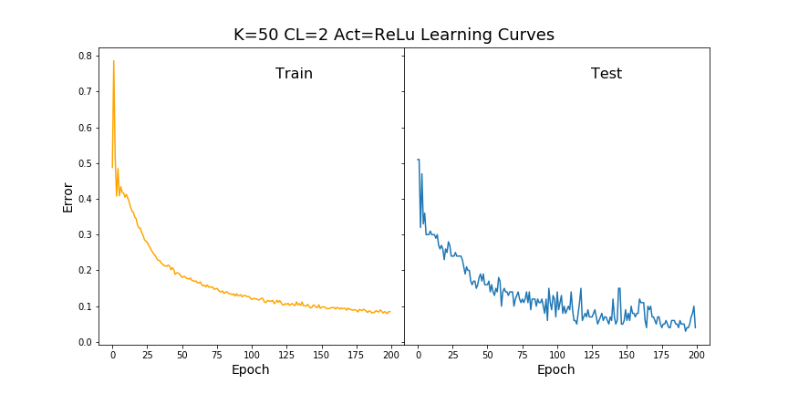
The learning curves for K=50, CL=2, and ReLu activation on the output layer are shown above.

In addition to the convolutional neural network, I also used a nearest neighbor regressor, which I thought would work well on this small scale within the grid of input parameters. However, outside of these simplistic settings, I do not expect this method to remain as accurate and fast. I used a three nearest neighbors regressor, with weights based on the distance to the three neighbors. With the three frequencies rescaled from zero to one, I used an L-2 distance metric.

FFR Results

Overall, all six models tested ran very similarly, which is encouraging. It seems the underlying function is not smooth. There is reason for this. The test samples are arranged by increasing eccentricity, but have varying inclinations. These two properties do not affect the phi frequency, but will alter the theta and r frequencies, therefore, making these curves oscillate. In the future, I would look into more drop out layers to try and smooth it out, pending a deeper analysis of the overfitting. The plot below shows the six models I tested, including the three nearest neighbors, compared to the actual fundamental frequencies. The solid lines are the actuals while the dotted lines are the predictions. The fundamental frequency in phi is smoother, and better reproduced by the models. The frequency in the radial direction fluctuates significantly; so do the model fits to this frequency.

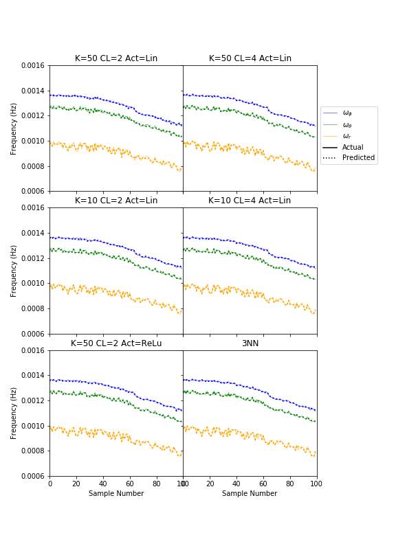
This plot shows the fit for each of the 6 models to each frequency. The frequencies in phi, theta, and r are shown in blue, green, and orange, respectively. The kernel size, convolutional layers, and output layer activation is indicated in the title of each plot with K, CL, and Act, respectively.

To compare these models further, I found the mean error and standard deviation on the error for each frequency from each model. Models 1 through 6 are in order: (K=50, CL=2, Act=Lin), (K=50, CL=4, Act=Lin), (K=10, CL=2, Act=Lin), (K=10, CL=4, Act=Lin), (K=50, CL=2, Act=ReLu), and 3NN. The higher the mean error, indicating the average difference from the true value, the worse the fit. The standard deviation on the error indicates the precision of the model. Smaller deviation means more precise with its predictions. The behavior between the frequencies is consistent, with the largest errors for the radial direction.

The best models turn out to be 2 and 4, i.e. (K=50, CL=4, Act=Lin) and (K=10, CL=4, Act=Lin). Both of these models have four convolutional layers. This is interesting, because they actually have less parameters to fit. The added convolutions must give a bit more information for the prediction. The precision on both of these measurements is quite good.

The worst model is model 1, (K=50, CL=2, Act=Lin). This has the least number of convolutional layers and the largest kernel. Lowering the kernel or adding layers improves the accuracy of the fit. Additionally, model 5 has the same number of layers and kernel size as model 1, with a different activation. This indicates replacing the linear activation on the output layer with a ReLu activation makes the model more precise. This makes sense. All of the outputs are greater than zero; ReLu activation reinforces this requirement.

CNN models 2 to 5 all perform better than nearest neighbors. This is quite encouraging for scaling. This means the faster query operation can also perform better.

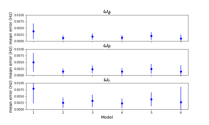
The mean errors and standard deviation on the errors for each model 1 through 6 are shown for each frequency.

Amplitude Spectrum Autoencoder (ASA)

ASA Methods

My methods for this part of the project were similar to the first. For the autoencoder, I tried a few different architectures. However, I landed on a convolutional autoencoder with two convolutional and pooling layers to encode the spectrum, and 3 layers with upscaling to decode it. The model with 4 encoding and 5 decoding layers returned worse results when compared to the original curves. The overfitting may have been the issue here. The kernel size for all convolutional layers was 20. The pooling layers pooled by a factor of 2, same with the upscaling layers. The convolutional layers had ReLu activation functions. The output layer had linear activation. It would be interesting to try this again with ReLu activation on the output layer.

ASA Results

Two images are seen at the beginning of this page showing the results of the autoencoder. I think calculating the error can actually be misleading for analyzing the autoencoder’s success. The key to this entire problem is to calculate harmonics of the fundamental frequencies from the amplitude spectral peaks. Therefore, the shape of the autoencoder and how it captures peaks are the most important factors for this project. However, for future projects, this will be a concern because The goal would be to reproduce the waveforms, which would require more precise amplitude spectrums. The peak structure is maintained pretty well. The dominant peaks are definitely captured. One major issue is that smaller peaks directly adjacent to larger peaks, are completely missed. These peaks can be very important for spectroscopic structure. An additional benefit of the autoencoder is that “fake” peaks resulting from effects of a discrete Fourier transform rather than from the actual signal begin to diminish, instead of remaining sharp.

Two more plots are shown below with eccentricities of 0.1 and 0.31 and inclinations of 0.13 and 0.47 radians. Both fits really do capture the main peak structure, but miss on the peaks adjacent to the main peaks. In general, the fluctuations from the discrete Fourier transforms are smoothed by the autoencoder. This may make it easier to categorize the binaries because the neural network and/or statistical methods will not get distracted by erroneous structure.

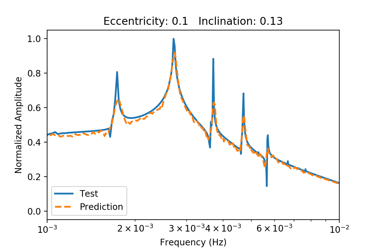
The amplitude spectrum is shown above for a binary with low eccentricity (0.1) and a lower inclination (0.13 radians). The prediction from the autoencoder is shown in dotted orange.

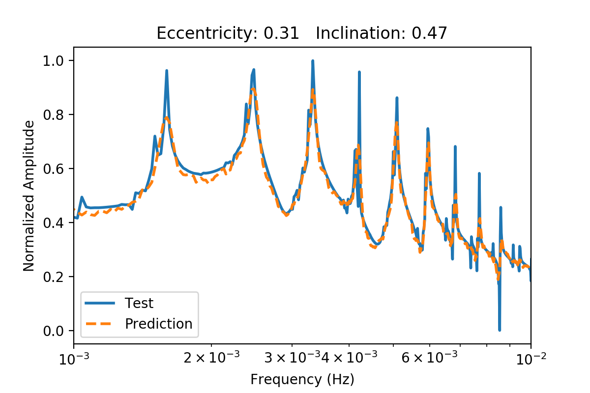
The amplitude spectrum is shown above for a binary with a higher eccentricity (0.31) and a lower inclination (0.47 radians). The prediction from the autoencoder is shown in dotted orange.

Future Work

This work can lead to many future investigations. The first thing I am going to do is add more parameters like masses of the small and large black hole as well as the spin of the large black hole. Also, I am going to further investigate with ReLu functions for the output layers. One aspect I would like to examine is a learning investigation comparing the Numerical Kludge to a faster waveform generator called the Advanced Analytical Kludge. The Numerical Kludge is more accurate in its waveform, but takes longer. It would be interesting to weigh the computational cost and the ability to train on many more waveforms against the slight loss in accuracy. I would also like to investigate this by adding a phase component, potentially making it 2D in the phase and amplitude. Additionally, griding the parameter space in non-uniform ways would be interesting to test. There are potentially more volatile areas of the parameter space that need to be gridded more densely than others. This will be good for memory and computational efficiency.

Another project I am beginning to look at is burying these signals in noise to see if the CNN can recognize the waveform and where it sits in the noise. Recognizing the waveform would be a binary classification task. I would train on injected waveforms as well as waveform-free noise time series. This would allow the CNN to train on both pure noise and embedded waveforms. Then, if the waveform is found, I would feed it into a second CNN to figure out where it is and give an initial parameter estimate. LISA will see tens of thousands of signals simultaneously. Therefore, the next step would be to not only bury the waveform in noise, but also within many other injected waveforms. I do not have a lot of faith in this last suggestion, but it is definitely something to test.

Finally, I want to further investigate the autoencoder. I would like to reduce this dimensionality with enough fidelity for a few reasons. One, I am investigating using gaussian processes to quickly generate new waveforms. This will only be possible with reduced dimensionality. Additionally, I am going to investigate lowering the dimensionality of the 17 dimensional phase space describing these waveforms. Using MCMC or other statistical techniques would be faster in a lower-dimensional encoded parameter space.