from eryn.ensemble import EnsembleSampler
from eryn.state import State
from eryn.prior import ProbDistContainer, uniform_dist
from eryn.utils import TransformContainer
from eryn.moves import GaussianMove, StretchMove, CombineMove
from eryn.utils.utility import groups_from_inds

import matplotlib.pyplot as plt
import numpy as np

# set random seed
np.random.seed(42)

import corner

Eryn Basic Tutorial

Eryn is an advanced MCMC sampler. It has the capability to run with parallel tempering, multiple model types, and unknown counts within each model type using Reversible-Jump MCMC techniques. Eryn is heavily based on emcee. The emcee base structure with the Ensemble Sampler, State objects, proposal setup, and storage backends is carried over into Eryn with small changes to account for the increased complexity. In a simple sense, Eryn is an advanced (and slightly more complicated) version of emcee.

In this tutorial, we will go through much of what is available in Eryn. We will start with a basic sampling operation to illustrate how to build and navigate common objects in Eryn. We will then scale up the complexity to understand how to use Eryn in different circumstances.

If you use Eryn in your publication, please cite the paper arXiv:2303.02164, its zenodo, and emcee. The documentation for Eryn can be found here: mikekatz04.github.io/Eryn. You will find the code on Github: github.com/mikekatz04/Eryn.

MCMC Basics

Here we will go through the basics of MCMC. For a better overall understanding of MCMC, see the Eryn paper: arXiv:2303.02164.

The goal of MCMC is to assess the posterior probablity on parameters \((\vec{\theta})\) from a model (\(\mathcal{M}\)), given some data \(y\): \(p(\vec{\theta}, \mathcal{M}|y)\). We can rewrite this probability using Bayes’ rule:

\[p(\vec{\theta}|y)=\frac{p(y|\vec{\theta}, \mathcal{M})p(\vec{\theta}, \mathcal{M})}{p(y|\mathcal{M})}\]

.

Here are the main pieces of the righthand side: * Posterior - \(p(\vec{\theta}|y)\): The probability distribution on the parameters, the main goal of MCMC. We will refer to this from now on as \(\pi(\vec{\theta})\). * Likelihood - \(p(y|\vec{\theta}, \mathcal{M})\): This is the surface that MCMC will sample (weighted by the prior). We will refer to the Likelihood. We will write this from now on as \(\mathcal{L}(\vec{\theta}, \mathcal{M})\). * Prior - \(p(\vec{\theta}, \mathcal{M})\): Prior probability on the parameters and the model chosen. * Evidence - \(p(y|\mathcal{M})\): The evidence is the integral of the numerator in the equation above integrated over all of the parameter space: \(\int_{\vec{\theta}_\mathcal{M}}\mathcal{L}(\vec{\theta}, \mathcal{M})d\vec{\theta}\). This will be referred to below as \(Z(\mathcal{M})\) (the evidence of model \(\mathcal{M}\)).

MCMC numerically draws samples from the posterior density by exploring the Likelihood surface weighted by the prior. In most MCMC applications, the evidence will be intractable and ignored as it is just a constant factor over all samples. There are methods to estimate the evidence that we will discuss below.

MCMC is special because of how it explores. Using a concept called “Detailed Balance,” walkers exploring the Likelihood surface preferentially move upwards, but probabilistically can move downwards. This allows for a full exploration of the peak of the Likelihood surface rather than just moving directly towards the highest point.

There are requirements to make this work properly that we will discuss below when we discsuss MCMC “moves” or “proposals.” At a basic level, also know as the Metropolis-Hastings algorithm, MCMC works like this: 1. It starts with a current point in parameter space, \(\vec{\theta}_t\). 2. The sampler proposes a new position for this walker: \(\vec{\theta}_{t+1}\). 3. It then accepts this new position with probabilty, \(\alpha\):

\[\min\left(1, \frac{\pi(\vec{\theta}_{t+1})q(\vec{\theta}_{t}|\vec{\theta}_{t+1})}{\pi(\vec{\theta}_{t})q(\vec{\theta}_{t+1}|\vec{\theta}_{t})}\right)\]

. 4. Repeat many times.

\(q\) is the proposal distribution to move from \(\vec{\theta}_{t}\) to \(\vec{\theta}_{t+1}\) or vice versa. If the proposal distribution is symmetric, the \(q\) distributions drop out and we are left with the fraction of posterior probabilities. We can see, in this case, if the new posterior probability is larger than the previous probability, the move will ALWAYS be accepted. If the new posterior probability is worse than the old probability, the move will be accepted with a probability equal to this fraction. Therefore, as the new value becomes worse and worse compared to the old value, the probability of acceptance decreases.

The Tree Metaphor

Before we get into using the sampler, we will discuss the “infamous” tree metaphor. It helped in thinking about the early creation of Eryn and has carried through to the end. Eryn is the Sindarin word for “forest” or “woods.” The purpose of this metaphor is to simplify the complex dimensionality associated with changing models and model counts in MCMC. We choose not to use “model” and “model counts” everywhere because those descriptions can quickly become confusing.

We start with a forest with a bunch of trees. These trees are the MCMC “walkers”. Each tree will have the same number of branches which is fixed throughout a sampling run (i.e. each walker has the same base setup). These branches are our different model types. For example, if you have a signal that is a combination of sine waves and Gaussians. In this case, you have two branches, one for the “sine wave” model and one for the “Gaussian” model. The number of Gaussians or sine waves is accounted for as the number of “leafs” on each branch. So, if 1 walker has 3 Gaussians and 2 sine waves, we can imagine this as a tree with two branches. The first branch for sine waves has 2 leaves and the second branch as 3 leaves for 3 Gaussians.

When we get to parallel tempering, you can imagine different forests at different temperatures, all having the same number of trees (walkers).

Getting Started with the Ensemble Sampler

Let’s start by running on a simple multivariate Gaussian likelihood:

\[\ln{\mathcal{L}}\propto -\frac{1}{2}(\vec{x} - \vec{\mu})^T \tilde{C}^{-1} (\vec{x} - \vec{\mu})\]

# Gaussian likelihood
def log_like_fn(x, mu, invcov):
    diff = x - mu
    return -0.5 * (diff * np.dot(invcov, diff.T).T).sum()

Add the initial settings: number of dimensions and number of walkers. Then, generate a covariance matrix for the given dimensionality for the likelihood and a set of means for each component of the Gaussian.

ndim = 5
nwalkers = 100

# mean
means = np.zeros(ndim)  # np.random.rand(ndim)

# define covariance matrix
cov = np.diag(np.ones(ndim))
invcov = np.linalg.inv(cov)

Next we will build our priors. For simplicity (and based on this problem), we will use a hyper-cube centered on the means with side length set to be 2 * lims. Eryn requires a class object as the prior with an logpdf method (similar to scipy.stats distributions). Eryn provides a helper class to aid in this process: `eryn.prior.ProbDistContainer <https://mikekatz04.github.io/Eryn/build/html/user/prior.html#prior-container>`__. This class takes a dictionary as input. In the simplest form, the keys are integers representing the index into the array of parameters and the values are the associated distributions: {index: distribution}. Eryn has a wrapper for the scipy.stats.uniform class that allows you to enter the start and stop points: `eryn.prior.uniform <https://mikekatz04.github.io/Eryn/build/html/user/prior.html#eryn.prior.uniform_dist>`__. For example, if we have a 3D space with uniform priors for all dimensions from -1 to 1, the input dictionary would look like this:

priors_in = {
    0: uniform_dist(-1, 1),
    1: uniform_dist(-1, 1),
    2: uniform_dist(-1, 1)
}

# set prior limits
lims = 5.0
priors_in = {i: uniform_dist(-lims + means[i], lims + means[i]) for i in range(ndim)}
priors = ProbDistContainer(priors_in)

In this case, we are not going to use really any of Eryn’s special capabilities. This will allow us to focus on how to navigate the sampler and deal with its output. Then we can add the fun stuff!

The object that directs everything in Eryn (like in emcee) is `eryn.ensemble.EnsembleSampler <https://mikekatz04.github.io/Eryn/build/html/user/ensemble.html#eryn.ensemble.EnsembleSampler>`__. It required arguments are number of walkers, dimensionality of inputs (for this simple case this is an integer), the log likelihood function, and the priors. Similar to emcee, you can add arguments and keyword arguments to the Likelihood function by providing the args and kwargs keyword arguments to the EnsembleSampler. In this case, we add the means and inverse of the covariance matrix as extra arguments.

ensemble = EnsembleSampler(
    nwalkers,
    ndim,
    log_like_fn,
    priors,
    args=[means, invcov],
)

Now we will get starting positions for our walkers by sampling from the priors using the rvs method of the ProbDistContainer and then evaluating the associated Likelihood and prior values. The rvs method is also called like in scipy.stats distributions.

# starting positions
# randomize throughout prior
coords = priors.rvs(size=(nwalkers,))

# check log_like
log_like = np.asarray([
    log_like_fn(coords[i], means, invcov)
for i in range(nwalkers)])
print(log_like)

# check log_prior
log_prior = np.asarray([
    priors.logpdf(coords[i])
for i in range(nwalkers)])
print(log_prior)

[-30.69858605 -27.88613553 -10.22294092 -14.70569247 -18.96300942
 -40.24777582 -18.73441074 -24.83741982 -29.01040764 -27.8427905
 -15.6395355  -37.63324244 -37.32945619 -23.65755241 -14.71578138
 -17.41587351 -10.60372232 -14.78508305 -16.44610878 -14.65807937
 -10.96569731 -21.07245692 -21.71012131 -11.7938995  -26.68678623
 -10.56139796 -21.07206293 -15.22766639 -21.70138195 -21.66486977
 -12.67496753 -16.03289018 -29.46929288 -26.72131899 -44.24698912
 -21.3584848  -19.77366496 -28.72150734  -5.84518648 -33.37118884
 -36.15731891 -25.26041351 -25.57594664 -12.25802303 -22.37039294
 -31.88982593 -15.35309536 -24.45627855 -22.46651653 -23.11210745
 -25.31311317 -14.36123373 -23.67409531 -23.41272599 -34.51272062
 -13.40386882 -42.6083427  -10.3819265  -33.56151466 -19.79275524
 -10.09464227 -17.63670509 -15.88594767  -1.5583328  -38.33786195
 -10.04251137 -22.92432228 -26.5383962  -29.02898281 -34.39747766
 -29.93610511 -43.67631032 -37.6288042  -26.57863213 -12.43201382
 -21.71339587 -24.98065915 -22.34629761 -28.53454745 -20.72808992
 -23.58751379 -13.39368888 -12.15662608 -32.82365756  -8.14075088
 -26.22668818 -20.43301692  -8.79050623 -23.10278803 -16.10581548
 -38.66327643 -21.96839538 -19.91765459 -10.73450427 -13.25399003
 -11.51642261 -12.99636574 -21.3527218  -33.90758502 -35.26045709]
[-11.51292546 -11.51292546 -11.51292546 -11.51292546 -11.51292546
 -11.51292546 -11.51292546 -11.51292546 -11.51292546 -11.51292546
 -11.51292546 -11.51292546 -11.51292546 -11.51292546 -11.51292546
 -11.51292546 -11.51292546 -11.51292546 -11.51292546 -11.51292546
 -11.51292546 -11.51292546 -11.51292546 -11.51292546 -11.51292546
 -11.51292546 -11.51292546 -11.51292546 -11.51292546 -11.51292546
 -11.51292546 -11.51292546 -11.51292546 -11.51292546 -11.51292546
 -11.51292546 -11.51292546 -11.51292546 -11.51292546 -11.51292546
 -11.51292546 -11.51292546 -11.51292546 -11.51292546 -11.51292546
 -11.51292546 -11.51292546 -11.51292546 -11.51292546 -11.51292546
 -11.51292546 -11.51292546 -11.51292546 -11.51292546 -11.51292546
 -11.51292546 -11.51292546 -11.51292546 -11.51292546 -11.51292546
 -11.51292546 -11.51292546 -11.51292546 -11.51292546 -11.51292546
 -11.51292546 -11.51292546 -11.51292546 -11.51292546 -11.51292546
 -11.51292546 -11.51292546 -11.51292546 -11.51292546 -11.51292546
 -11.51292546 -11.51292546 -11.51292546 -11.51292546 -11.51292546
 -11.51292546 -11.51292546 -11.51292546 -11.51292546 -11.51292546
 -11.51292546 -11.51292546 -11.51292546 -11.51292546 -11.51292546
 -11.51292546 -11.51292546 -11.51292546 -11.51292546 -11.51292546
 -11.51292546 -11.51292546 -11.51292546 -11.51292546 -11.51292546]

Because we are in the unit cube, the prior values are constant.

Now, we can run the sampler using the run_mcmc method on the EnsembleSampler class. It first takes as an argument an array of the starting positions (or a State object which we will cover below). We also must provide the number of steps as the second argument. Helpful kwargs (not all inclusive):

• burn: Perform a burn in for a certain number of proposals.

• progress: If True, show the progress as the sampler runs.

• thin_by: How much to thin the chain directly before storage.

The total number of proposals the sampler will do is nsteps * thin_by. It will store nsteps samples.

nsteps = 500
# burn for 1000 steps
burn = 100
# thin by 5
thin_by = 5
out = ensemble.run_mcmc(coords, nsteps, burn=burn, progress=True, thin_by=thin_by)

100%|████████████████████████████████████████| 100/100 [00:00<00:00, 247.07it/s]
100%|██████████████████████████████████████| 2500/2500 [00:09<00:00, 261.19it/s]

Similar to emcee, all of the sampler information is stored in a backend object. In the default case, this backend is `eryn.backends.Backend <https://mikekatz04.github.io/Eryn/build/html/user/backend.html#eryn.backends.Backend>`__. To retrieve the samples from the backend, you call the get_chain method. This will return a dictionary with keys at the omdel names and a 5-dimensional array per model, which can be intimidating. We will cover that array just below. For now, just focus on the output of the sampler.

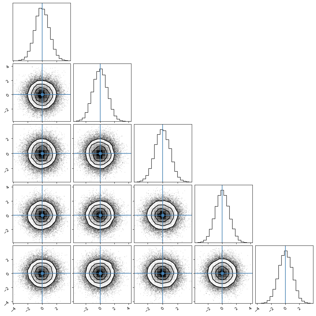
We will first generate corner plot. In this initial example, we have not defined branch names, therefore, the sampler has assigned our problem default branch names model_0,…,model_n.

samples = ensemble.get_chain()['model_0'].reshape(-1, ndim)
corner.corner(samples, truths=means)

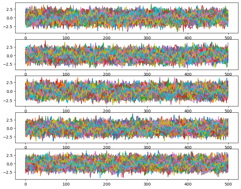
Now we will plot the chains.

#### Chains
fig, ax = plt.subplots(ndim, 1)
fig.set_size_inches(10, 8)
for i in range(ndim):
    for walk in range(nwalkers):
        ax[i].plot(ensemble.get_chain()['model_0'][:, 0, walk, :, i])

Backend Objects

Backends are where all of the information in the sampler is stored as it runs. It is from these backends that samples are retrieved for plotting. You can find the documentation for the Backend objects here. Here, we will go through the most commonly used functions from the backend: * get_chain: retrieve all of the samples stored over the course of the sampling run. * get_log_like: retrieve the log of the Likelihood for each sample. * get_log_prior: retrieve the log of the prior for each sample. * get_a_sample: retrieve a state object from a specific iteration. get_last_sample may be more common. It is just a specific example of get_a_sample for the last sample.

Many (but not all) of the methods from the backend object are also raised to the level of sampler. So you can either call EnsembleSampler.backend.method or EnsembleSampler.method and it will be equivalent.

Common properties to get from the backend: * shape: returns a dictionary with keys for each branch name and values as tuples representing the specific shape for each model (this shape will not include the nsteps outer dimension. * iteration: number of stored iterations in the backend.

Now we will get the likelihood and prior. Notice the shape of the Likelihood is (nsteps, ntemps, nwalkers) (in this example we have 1 temperature). This will always be the shape of quantities that are a single value per walker (e.g. Likelihood, prior, posterior).

ll = ensemble.backend.get_log_like()
lp = ensemble.backend.get_log_prior()

print(f"Number of iterations {ensemble.backend.iteration}")
# equivalent to ensemble.get_log_like() and ensemble.get_log_prior()
print(ll.shape, ll, lp)

Number of iterations 500
(500, 1, 100) [[[-1.05297225 -2.81695595 -0.80839791 ... -1.30449907 -2.65001331
   -1.72492908]]

 [[-3.51878996 -0.89787788 -4.49356178 ... -4.65518146 -3.7436319
   -1.66068016]]

 [[-2.03059694 -1.49585829 -3.90577462 ... -1.04656098 -2.0396035
   -0.80658449]]

 ...

 [[-1.73887276 -2.27535667 -1.36789573 ... -1.19099689 -2.72232295
   -5.43958501]]

 [[-1.44427868 -1.05581352 -4.30749439 ... -1.85688564 -2.11343788
   -2.24766066]]

 [[-0.6654815  -2.28154314 -2.00102494 ... -1.6139005  -1.08899932
   -2.1398411 ]]] [[[-11.51292546 -11.51292546 -11.51292546 ... -11.51292546 -11.51292546
   -11.51292546]]

 [[-11.51292546 -11.51292546 -11.51292546 ... -11.51292546 -11.51292546
   -11.51292546]]

 [[-11.51292546 -11.51292546 -11.51292546 ... -11.51292546 -11.51292546
   -11.51292546]]

 ...

 [[-11.51292546 -11.51292546 -11.51292546 ... -11.51292546 -11.51292546
   -11.51292546]]

 [[-11.51292546 -11.51292546 -11.51292546 ... -11.51292546 -11.51292546
   -11.51292546]]

 [[-11.51292546 -11.51292546 -11.51292546 ... -11.51292546 -11.51292546
   -11.51292546]]]

5-dimensional Arrays

The chain information is returned as a dictionary with keys as the branch names and values as 5-dimensional arrays: (nsteps, ntemps, nwalkers, nleaves_max, ndim). For clarity: * nsteps: number of sampler iterations stored (time evolution of each forest) * ntemps: number of temperatures (which forest you are in) * nwalkers: number of walkers (which tree) * nleaves_max: maximum number of model counts or leaves for each specific branch. * ndim: number of parameters describing a single model or leaf.

In our simple example, we have 1 temperature and our maximum leaf count is 1.

# getting the chain
samples = ensemble.get_chain()

# same as
# samples = enseble.backend.get_chain()
print(type(samples), samples.keys(), samples["model_0"].shape)

<class 'dict'> dict_keys(['model_0']) (500, 1, 100, 1, 5)

We can also get the shape information direct from the backend:

ensemble.backend.shape

{'model_0': (1, 100, 1, 5)}

State Objects

Now, we are going to look at `State <https://mikekatz04.github.io/Eryn/build/html/user/state.html#eryn.state.State>`__ objects. They carry the current information throughout the sampler about the current state of the sampler. In our simple example, we can examine the current coordinates, likelihood, and prior values.

Output from the sampler above is the last state of the sampler out. This will include any additional objects passed through the sampler like BranchSupplemental objects that we will explain below.

Another way to retrieve the last state is from the backend. That is what we will do here. However, please note, that supplimental information (discussed below) is not stored in the backend, so the state that is returned from the backend will have information that is stored in the backend, but not supplimental information that was passed through the sampler at runtime.

last_state = ensemble.backend.get_last_sample()
print(type(last_state))

<class 'eryn.state.State'>

We can access the Likelihood and prior values as State.log_like and State.log_prior. We can also ask the state to give use the posterior probability with the get_log_posterior method. Note that shape of these values is (ntemps, nwalkers). This is because State objects represent one moment in time in the sample, so they do not have the nsteps outer dimension that the backend has.

print(out.log_like.shape, out.log_like, out.log_prior, out.get_log_posterior())

(1, 100) [[-0.6654815  -2.28154314 -2.00102494 -4.41852808 -1.87391204 -3.05035603
  -1.47197889 -3.04722716 -3.8519063  -2.53028792 -1.47895075 -0.91435392
  -4.67615627 -6.59494035 -3.09579563 -2.31956089 -3.61486196 -1.12447462
  -2.1692713  -4.54813706 -5.47761491 -1.81600973 -2.57141612 -3.18369399
  -8.03114163 -4.03929851 -1.37835437 -1.41370852 -2.04192051 -4.24060107
  -1.81791365 -1.43145056 -1.01976309 -1.08419629 -3.29498179 -2.08090042
  -3.03457142 -0.97839311 -1.45783438 -0.54860516 -0.39096809 -1.63453914
  -2.05034555 -1.13275529 -2.13057916 -3.21847262 -2.14804885 -2.15556008
  -1.92686111 -1.99795709 -0.35164059 -1.21098077 -1.21647944 -1.15304968
  -3.4313149  -4.70693915 -1.4318716  -4.84488379 -2.02338003 -2.07328961
  -2.98861309 -1.0448529  -4.76536477 -1.86707428 -1.24040534 -1.52161672
  -0.93361207 -1.10290796 -1.69669336 -0.98189704 -5.90223547 -3.3408396
  -2.12094704 -3.14709346 -0.37990706 -1.48720061 -3.15361028 -1.1595534
  -1.80055637 -1.59197714 -3.34129599 -1.36805722 -2.01708067 -3.58699943
  -2.32689704 -2.58811303 -2.7197202  -2.05348442 -1.2112424  -1.3357544
  -1.65449106 -1.68322549 -1.04792421 -1.13391508 -2.31811812 -2.46163754
  -5.10129065 -1.6139005  -1.08899932 -2.1398411 ]] [[-11.51292546 -11.51292546 -11.51292546 -11.51292546 -11.51292546
  -11.51292546 -11.51292546 -11.51292546 -11.51292546 -11.51292546
  -11.51292546 -11.51292546 -11.51292546 -11.51292546 -11.51292546
  -11.51292546 -11.51292546 -11.51292546 -11.51292546 -11.51292546
  -11.51292546 -11.51292546 -11.51292546 -11.51292546 -11.51292546
  -11.51292546 -11.51292546 -11.51292546 -11.51292546 -11.51292546
  -11.51292546 -11.51292546 -11.51292546 -11.51292546 -11.51292546
  -11.51292546 -11.51292546 -11.51292546 -11.51292546 -11.51292546
  -11.51292546 -11.51292546 -11.51292546 -11.51292546 -11.51292546
  -11.51292546 -11.51292546 -11.51292546 -11.51292546 -11.51292546
  -11.51292546 -11.51292546 -11.51292546 -11.51292546 -11.51292546
  -11.51292546 -11.51292546 -11.51292546 -11.51292546 -11.51292546
  -11.51292546 -11.51292546 -11.51292546 -11.51292546 -11.51292546
  -11.51292546 -11.51292546 -11.51292546 -11.51292546 -11.51292546
  -11.51292546 -11.51292546 -11.51292546 -11.51292546 -11.51292546
  -11.51292546 -11.51292546 -11.51292546 -11.51292546 -11.51292546
  -11.51292546 -11.51292546 -11.51292546 -11.51292546 -11.51292546
  -11.51292546 -11.51292546 -11.51292546 -11.51292546 -11.51292546
  -11.51292546 -11.51292546 -11.51292546 -11.51292546 -11.51292546
  -11.51292546 -11.51292546 -11.51292546 -11.51292546 -11.51292546]] [[-12.178406967597018 -13.794468601537229 -13.51395040804473
  -15.931453545910662 -13.386837504796224 -14.563281497846829
  -12.984904356428126 -14.560152628566094 -15.364831763416989
  -14.043213387296886 -12.991876210506318 -12.427279383435607
  -16.18908173602542 -18.107865819910735 -14.608721090901623
  -13.832486351401688 -15.12778742254714 -12.637400087040206
  -13.682196761468905 -16.061062522948745 -16.99054037739138
  -13.328935193719195 -14.084341581952058 -14.696619458753926
  -19.544067098137223 -15.552223973129747 -12.89127983919111
  -12.926633980338917 -13.55484597643607 -15.753526531972273
  -13.330839113958634 -12.944376020031633 -12.532688554298963
  -12.597121756200298 -14.807907257937872 -13.593825884034455
  -14.547496880273862 -12.491318574369066 -12.970759842526956
  -12.061530625801362 -11.903893550359193 -13.147464607768942
  -13.563271019780707 -12.64568075132453 -13.643504626290895
  -14.731398085093454 -13.660974318785833 -13.668485545961143
  -13.439786571171963 -13.510882553516781 -11.864566059032157
  -12.72390623089636 -12.729404901485783 -12.665975147003136
  -14.94424036264724 -16.219864618156716 -12.944797066539389
  -16.357809250310932 -13.536305491515654 -13.586215078293383
  -14.501538559296131 -12.557778368205309 -16.278290231060463
  -13.37999974857351 -12.753330808148338 -13.034542185913606
  -12.44653753837222 -12.61583342786152 -13.209618824491073
  -12.494822509135583 -17.415160934688622 -14.8537650614948
  -13.633872503903893 -14.66001892478048 -11.892832526613594
  -13.000126072062562 -14.666535740104562 -12.672478860022272
  -13.313481837705911 -13.104902607647315 -14.854221450723335
  -12.880982689335216 -13.530006134397748 -15.099924895847023
  -13.839822509144446 -14.101038497292365 -14.232645664310798
  -13.566409885481924 -12.724167865929159 -12.848679866185286
  -13.167416523641707 -13.196150950789018 -12.560849676395932
  -12.646840543492647 -13.831043581839076 -13.974563002223718
  -16.614216117226597 -13.126825968142406 -12.601924782141412
  -13.65276656606936]]

Branches

State objects store quantities at are single values per walker directly in the state as shown above (e.g. State.log_like). Information that gets down to the individual branch (or model type) level is stored in a `Branch <https://mikekatz04.github.io/Eryn/html/user/state.html#eryn.state.Branch>`__ object. These Branch objects are stored in a dictionary within the State object with keys as branch names and values as the Branch object associated with that branch name. The branch objects can be accessed as state.branches[model_name]. With in the branch object, the coordinates are stored. A few other things are stored, but we will get to that later. If you want a dictionary with keys at the branch names and values as the current coordinates, you can also use the property: state.branches_coords.

last_state.branches

{'model_0': <eryn.state.Branch at 0x134b34800>}

last_state.branches["model_0"].coords

# same as
# last_state.branches_coords["model_0"]

array([[[[ 0.78336101, -0.50304083, -0.16554043,  0.38717246,
          -0.53567929]],

        [[ 1.67992539,  0.45789611,  0.71044046,  0.99561671,
          -0.18785587]],

        [[ 1.58942687, -0.98468048, -0.23409897, -0.34754982,
           0.5749637 ]],

        [[-1.51043746,  1.46761376, -1.36652826,  0.13575554,
           1.58616381]],

        [[ 0.56687718, -0.71412812, -1.07272873,  0.90290266,
          -0.9749437 ]],

        [[-0.26148892, -0.32754323,  2.05336273,  0.43505825,
           1.23267062]],

        [[-0.11388586,  0.97965383,  1.18803374, -0.55536628,
           0.50140833]],

        [[ 0.97231495, -1.80168105, -0.87750463,  0.55941876,
           0.9055604 ]],

        [[ 0.93206222,  0.61099548,  0.22893838, -0.06397951,
           2.53085973]],

        [[ 1.78123828,  0.29397075,  0.87720694, -0.51235873,
          -0.87712242]],

        [[-0.0915609 , -0.06094217,  0.39300579,  0.27838045,
          -1.6473782 ]],

        [[ 0.6848448 ,  0.37394608,  0.43214013,  0.80375073,
          -0.62217316]],

        [[ 1.78087387, -0.37379556, -1.70695828,  0.98429392,
          -1.46919589]],

        [[ 0.87912662,  0.80736483,  2.84535279, -1.02691072,
          -1.61697279]],

        [[-1.59413254, -1.14139239, -0.70216385,  0.56814835,
           1.23763059]],

        [[-1.8783785 , -0.93419666,  0.25561706, -0.41370698,
          -0.03998814]],

        [[-0.43668379, -0.39311608, -0.07642243,  2.43586086,
           0.97223065]],

        [[ 0.00745957, -0.21236731,  0.23184676,  0.8907263 ,
           1.16475211]],

        [[-1.7308126 ,  0.62439654,  0.69996634,  0.52028448,
          -0.43853217]],

        [[-2.30865891,  0.92696939, -0.98209765,  0.4834703 ,
          -1.30722477]],

        [[ 2.07144626, -0.56432505, -0.29089771,  1.32751881,
           2.1210728 ]],

        [[ 0.25274812,  0.9270326 , -0.58971747,  0.75561133,
           1.33792123]],

        [[ 0.05336995, -1.51405245,  0.06533858, -0.93630816,
          -1.40238616]],

        [[ 0.10136621, -1.01709496,  0.08910818, -0.52223649,
           2.2454308 ]],

        [[-0.86197169,  3.73127788,  1.07000261, -0.29443113,
          -0.40651963]],

        [[-1.81087754, -1.31763714,  1.12761906, -0.55144102,
          -1.21964748]],

        [[ 0.72082232, -0.66783269, -0.61110439, -0.05759876,
          -1.18926752]],

        [[-0.31039828, -0.84006455, -0.7555078 , -0.88418758,
           0.82023276]],

        [[-1.15032279, -1.28216431,  0.19945317,  0.9670416 ,
          -0.37643346]],

        [[-0.20656978, -1.09247869, -0.83026592, -0.29333812,
          -2.54354725]],

        [[ 0.0506733 ,  1.58235446, -1.0591977 , -0.01318246,
          -0.08567564]],

        [[ 1.00402466, -1.09280401, -0.57272931, -0.10612996,
          -0.56686201]],

        [[ 0.63470563, -0.29598879,  0.03616789,  1.20713821,
          -0.3009565 ]],

        [[ 0.69564655,  0.26928194,  1.15389273,  0.12383051,
           0.51493035]],

        [[-1.79119556,  0.69120098,  0.01019032, -1.21449347,
           1.19529285]],

        [[ 0.39078543,  1.32386668,  1.4771604 ,  0.02665296,
          -0.27157202]],

        [[ 1.66344411,  1.40855699, -0.2227286 , -0.03021349,
           1.12585205]],

        [[ 0.0358304 ,  0.67413575, -0.6791267 , -0.17160254,
           1.00517803]],

        [[-0.66454531,  0.44931894,  1.2731242 ,  0.80140622,
           0.09520302]],

        [[ 0.08417592, -0.2045363 , -0.81677496,  0.60685038,
           0.11358217]],

        [[-0.41939285,  0.56655054, -0.45246425,  0.12320174,
          -0.25527187]],

        [[ 0.02585738,  1.4670955 ,  0.71912218,  0.7720434 ,
          -0.05341122]],

        [[ 1.29611737,  0.1748023 ,  0.4372776 , -0.68897449,
          -1.3131327 ]],

        [[ 0.24317085,  0.05633037,  0.50847769, -1.16816417,
          -0.76160903]],

        [[-0.43456796,  0.81744538,  0.64783055,  1.33848598,
          -1.09218265]],

        [[-0.19003503,  1.0901105 , -1.68079509, -0.42874181,
           1.48445254]],

        [[-0.09533596,  1.1585624 , -0.28324105,  1.41256148,
          -0.93230171]],

        [[ 0.30259333, -1.2291636 ,  1.14969874,  1.02255485,
          -0.58419916]],

        [[-0.4221966 ,  0.85477946,  0.25227351,  0.96312104,
          -1.39770535]],

        [[-1.0401763 ,  0.6414978 ,  0.55821906, -0.14829119,
          -1.47269454]],

        [[-0.10152982,  0.38256367,  0.08807142,  0.43429676,
           0.59181726]],

        [[ 0.05120369, -0.77512143,  1.14463123, -0.23983033,
           0.67143671]],

        [[ 1.50082842, -0.30584941,  0.20683388, -0.03483413,
           0.20720856]],

        [[-1.08598898,  0.22080208, -0.64865562,  0.40682697,
           0.70122139]],

        [[-0.64175924, -1.58143259,  0.89952925,  1.54536517,
          -0.86749033]],

        [[ 1.06019685, -0.04449809,  1.47050671,  1.04282887,
          -2.24454869]],

        [[ 1.32891118,  0.38437228, -0.71091403, -0.65667314,
           0.11566271]],

        [[-1.52706537,  0.56474267, -0.76715602, -2.42312996,
           0.76080056]],

        [[-1.67036294, -0.28564342, -0.21110799, -0.14839688,
          -1.05283774]],

        [[ 0.05478405, -0.08082125,  0.1447414 , -1.98462828,
           0.42112513]],

        [[-1.21974939, -1.10592271,  1.67658838, -0.49570422,
           0.45793154]],

        [[-1.02752867, -0.5590723 , -0.54126603, -0.48664511,
          -0.43764875]],

        [[ 0.66773172,  0.82481843, -0.15349943,  2.88049842,
          -0.28931849]],

        [[-1.31243376,  1.3452211 ,  0.40682334,  0.18493076,
           0.04839187]],

        [[ 0.50253895,  0.19130782,  0.11088476,  0.56778619,
          -1.36271421]],

        [[ 0.5242914 , -0.99162198,  0.9547818 ,  0.25692932,
          -0.89856378]],

        [[ 0.15281554,  0.77735714, -1.11311344, -0.01051167,
           0.02134045]],

        [[ 0.06119311,  1.17510522, -0.52670296, -0.42278451,
          -0.60418234]],

        [[ 0.24963427,  1.1611201 ,  1.10664802, -0.70071643,
          -0.51691024]],

        [[ 0.89998806, -0.3590725 , -0.0173904 ,  0.94144735,
           0.37182924]],

        [[ 1.37866043, -1.28597385, -0.24976022,  0.42612563,
           2.82950074]],

        [[ 1.72487348, -0.00682858, -1.25268318,  1.29240179,
           0.68332019]],

        [[-0.05155055, -1.9316834 ,  0.34874628, -0.4050601 ,
           0.47131539]],

        [[-0.68665177, -1.32277562,  1.62515034, -1.04049481,
           0.59094657]],

        [[ 0.29061988,  0.28060227,  0.45655932, -0.60961052,
           0.12862806]],

        [[-1.0491748 , -0.19942752, -0.27318093,  0.79095823,
          -1.06471564]],

        [[-1.32490203, -2.01371249, -0.69586741, -0.07780255,
           0.08082376]],

        [[ 0.902882  , -0.40395368, -0.57161503, -0.6188732 ,
           0.79434534]],

        [[ 1.33174975, -0.08962046, -0.40607314,  1.28465644,
          -0.0654673 ]],

        [[ 0.99906271, -1.14535375, -0.31550719,  0.49069006,
          -0.73052807]],

        [[-1.31724964,  0.01639082, -0.97773904,  1.77949826,
           0.90806883]],

        [[ 0.60840415,  0.35765918,  1.09470711,  0.24921034,
           0.98871092]],

        [[ 1.15249127, -1.04587488,  0.68114623, -0.44485005,
           0.97479187]],

        [[-0.41527236,  1.18904736, -1.55784624, -1.77663656,
           0.06626997]],

        [[-0.69748913,  0.91203846,  0.65645409,  0.67068651,
           1.56675987]],

        [[ 0.13570414,  0.561949  , -0.00650889,  2.20041901,
          -0.01172908]],

        [[ 0.006941  , -1.27228794, -0.85989137,  1.46663793,
          -0.96448725]],

        [[-1.49410352, -0.02103752, -0.89929408,  0.99124781,
          -0.28788692]],

        [[ 1.21738227, -0.20578794,  0.62613854, -0.54711243,
          -0.45468127]],

        [[-1.35998576,  0.23620079,  0.19631993,  0.81886101,
          -0.23891811]],

        [[-0.32009865, -0.99200186, -0.58326714,  1.2244503 ,
          -0.61884746]],

        [[ 0.30593953, -0.54655862, -1.54046119,  0.45128582,
          -0.63043325]],

        [[ 0.92726937,  0.10223362,  0.89663029,  0.12669414,
           0.63684452]],

        [[-0.74616171,  0.41006412, -0.4589307 ,  0.09501266,
          -1.15033712]],

        [[ 0.21188577, -0.69703418,  0.09822929,  1.27225746,
           1.57391104]],

        [[-0.3775653 ,  1.3247288 , -1.12052205, -0.0951038 ,
          -1.32710163]],

        [[-2.55808909,  0.61767066,  0.28774531,  1.08037741,
           1.42380889]],

        [[-0.05488234,  1.12340336,  0.8862303 , -0.52472562,
           0.9497435 ]],

        [[-0.35200129,  0.36531645,  0.22484955,  1.08386021,
           0.83386291]],

        [[-1.83839054,  0.67436706, -0.56586041,  0.24858485,
           0.2514738 ]]]])

Parallel Tempering

Adding tempering to our problem is straight forward. It will effectively just take the ntemps dimension that was 1 above and stretch it to the number of temperatures desired. We add tempering information by providing the tempering_kwargs argument to the EnsembleSampler. The tempering kwargs documentation can be found here because they are the kwargs that go into the initialization of the temperature controller: `eryn.moves.tempering.TemperatureControl <https://mikekatz04.github.io/Eryn/html/user/temper.html#eryn.moves.tempering.TemperatureControl>`__.

The simplest thing to do is to provide the number of temperatures. In this case, we just pass ntemps in a dictionary. You can also provide a direct array of betas (inverse temperatures). Under the hood, if only ntemps is passed (not betas), the sampler will use the `eryn.moves.tempering.make_ladder <https://mikekatz04.github.io/Eryn/html/user/temper.html#eryn.moves.tempering.make_ladder>`__ function. We will go all thr way through to the MCMC run. Notice that we are once again just passing coords as an array to start the sampling. We could also pass a State object.

What does tempering actual do? The inverse temperature, \(\beta=1/T\), is attached as an exponent on the Likelihood. The posterior probability as a function of inverse temperature is given by,

\[\pi_\beta(\vec{\theta}, \mathcal{M})\propto (\mathcal{L}(\vec{\theta}, \mathcal{M}))^\beta p(\vec{\theta},\mathcal{M}).\]

If \(T=1\rightarrow \beta=1\), we are probing our TARGET distribution.

If \(T=\infty\rightarrow \beta=0\), we are probing the PRIOR distribution. In this case, the Likelihood surface is effectively flat.

Temperatures in between represent the gradual flattening of the target Likelihood surface towards the flat surface at infinite temperature. During sampling, we look at the log of the Likelihood, so the inverse temperature becomes a multiplicative factor:

\[\ln\pi_\beta(\vec{\theta}, \mathcal{M})\propto\beta\ln\mathcal{L}(\vec{\theta}, \mathcal{M})\]

Tempering is useful for multimodal distributions and to improve mixing in your chains. This mixing is created by swapping between rungs on our temperature ladder. After each sampler step, swaps are proposed starting at the two highest temperatures and iterating down until we reach the two lowest temperatures. This ensures as higher temperature chains find better Likelihood values, these values and positions are passed toward the cold chain (\(\beta=1\)). The swaps between chains are accepted with fraction, \(\alpha_T\):

\[\alpha_T = \min\left(1, \left[\frac{\mathcal{L_{\beta_1}}}{\mathcal{L_{\beta_2}}}\right]^{\beta_1 - \beta_2}\right).\]

We can see from this how swapping is similar to the Metropolis-Hastings acceptance setup.If \(\beta_1 > \beta_2\) (or \(T_1 <T_2\)), the exponent is positive. In this case, if \(\mathcal{L_{\beta_1}} > \mathcal{L_{\beta_2}}\), the swap will always be accepted because we want the better likelihood to go to higher \(\beta\) (or lower \(T\)). If \(\mathcal{L_{\beta_1}} < \mathcal{L_{\beta_2}}\), the swap is accepted with a probability that reflects difference in the Likelihoods just like discussed above.

# set up problem
ndim = 5
nwalkers = 100
ntemps = 10

# fill kwargs dictionary
tempering_kwargs=dict(ntemps=ntemps)

# randomize throughout prior
coords = priors.rvs(size=(ntemps, nwalkers,))

# initialize sampler
ensemble_pt = EnsembleSampler(
    nwalkers,
    ndim,
    log_like_fn,
    priors,
    args=[means, cov],
    tempering_kwargs=tempering_kwargs
)

nsteps = 500
# burn for 1000 steps
burn = 1000
# thin by 5
thin_by = 5
ensemble_pt.run_mcmc(coords, nsteps, burn=burn, progress=True, thin_by=thin_by)

100%|███████████████████████████████████████| 1000/1000 [00:15<00:00, 66.39it/s]
100%|███████████████████████████████████████| 2500/2500 [00:37<00:00, 66.02it/s]

<eryn.state.State at 0x134c6b350>

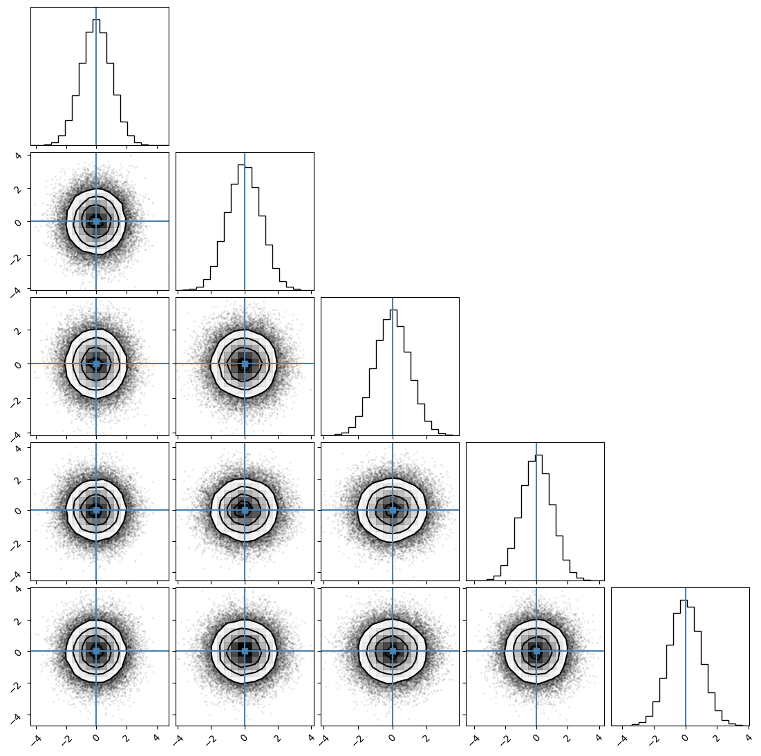
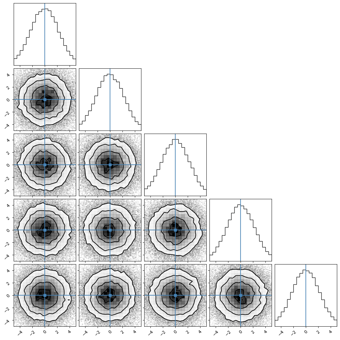
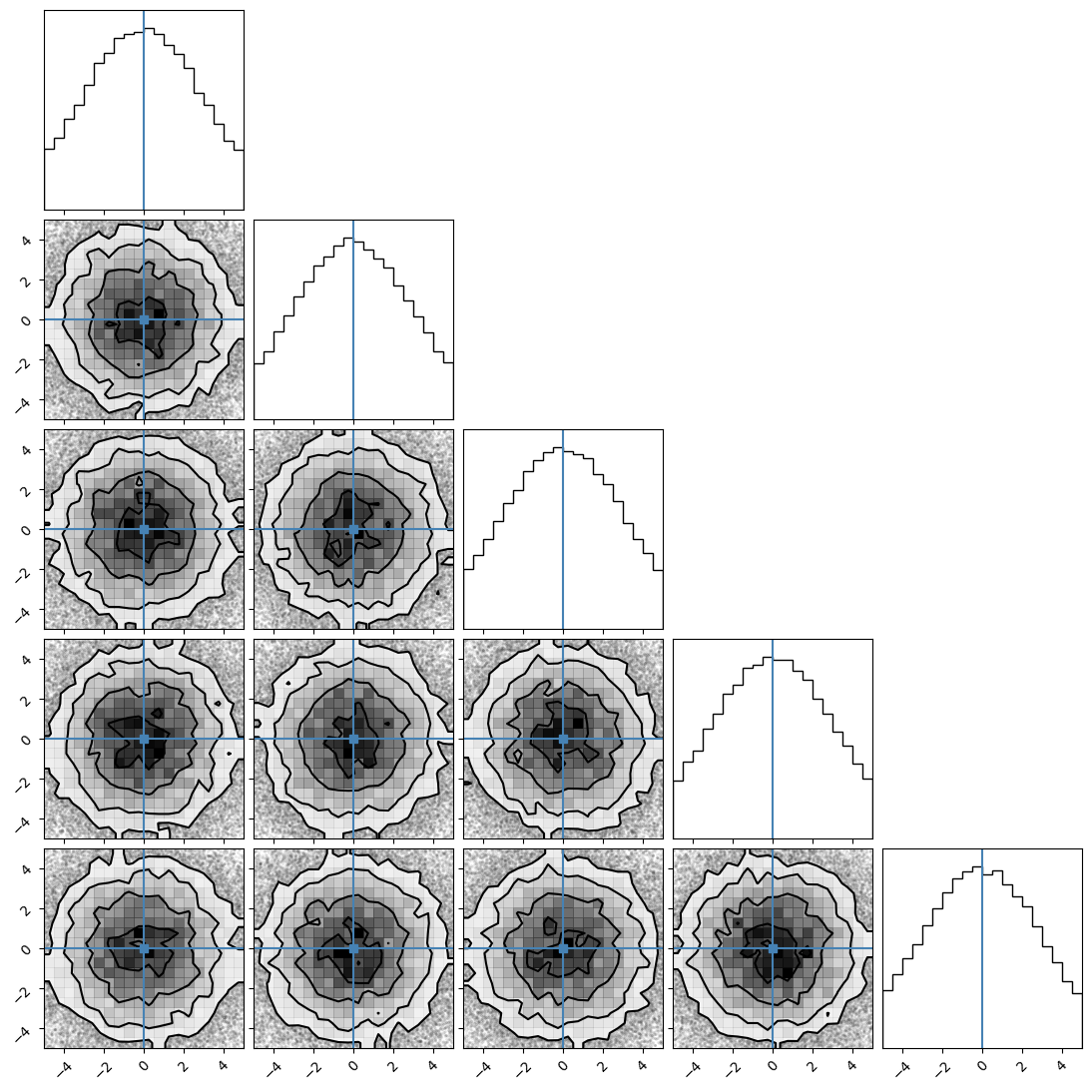
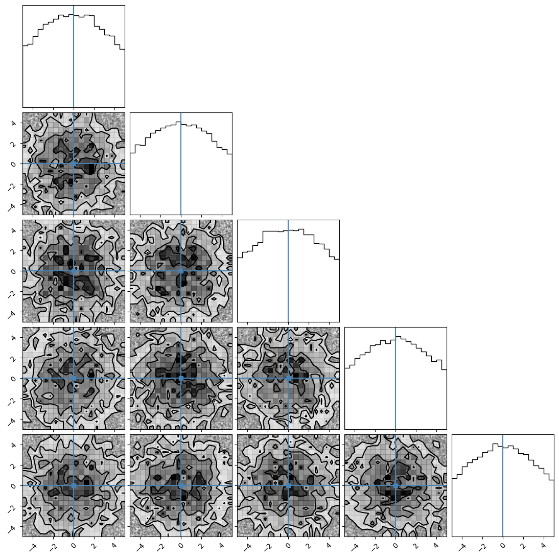
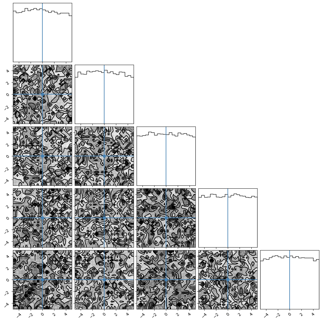
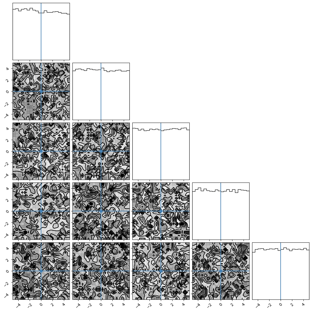
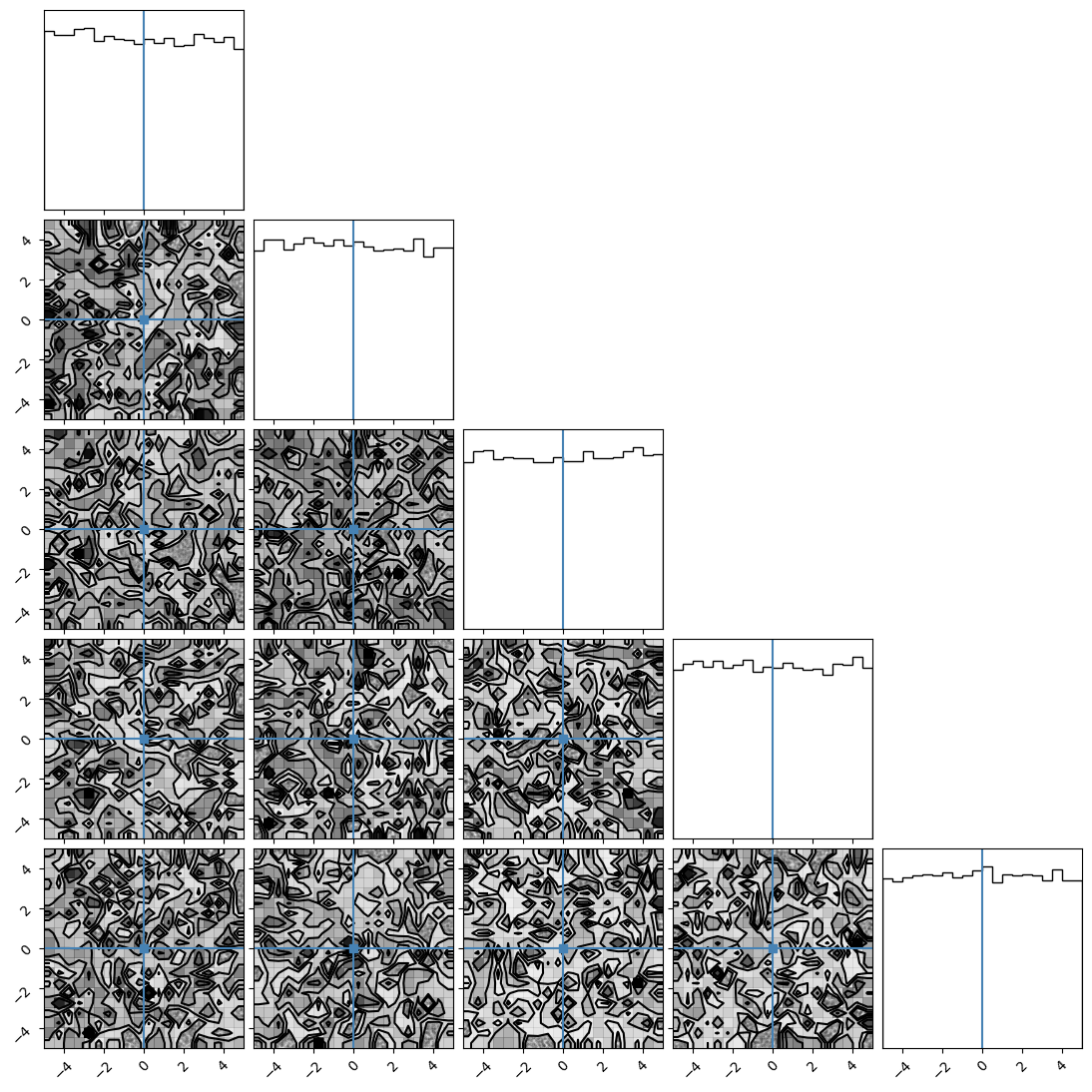
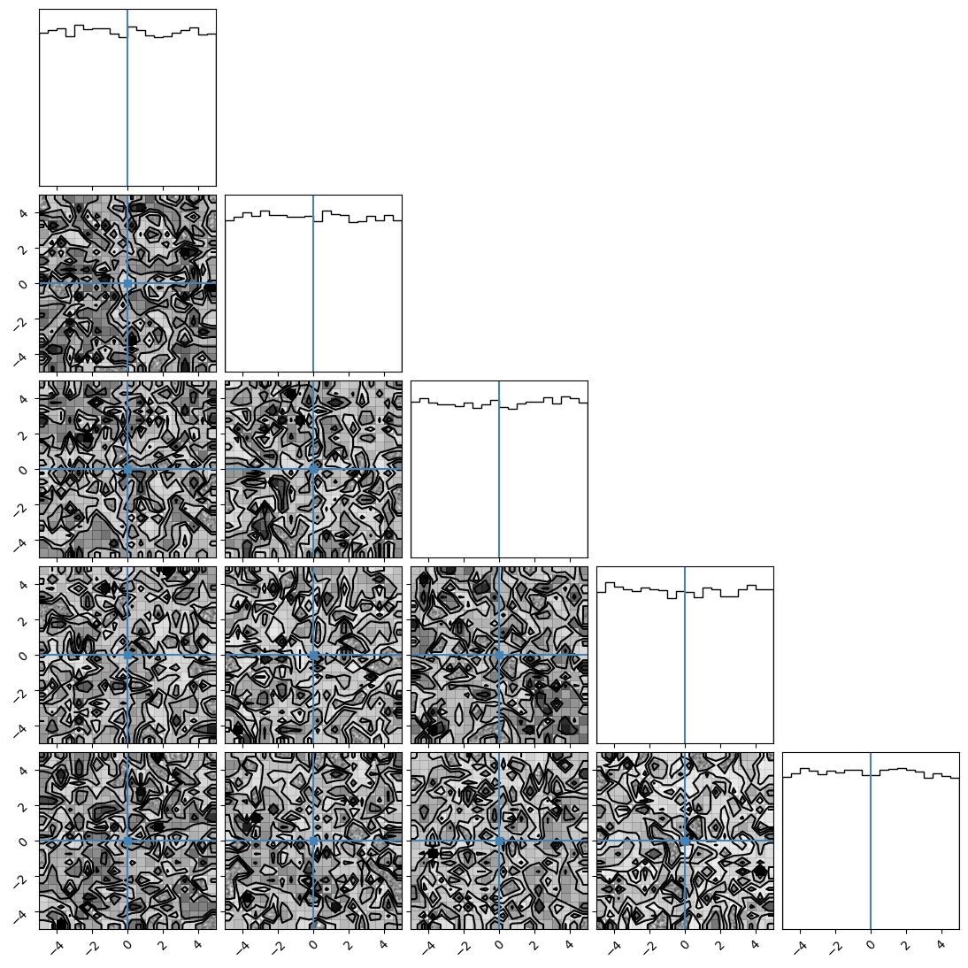
We can plot our samples at different temperatures and see the differences in action.

for temp in range(ntemps):
    print(temp + 1)
    samples = ensemble_pt.get_chain()['model_0'][:, temp].reshape(-1, ndim)
    corner.corner(samples, truths=np.full(ndim, 0.0))

1
2
3
4
5
6
7
8
9
10

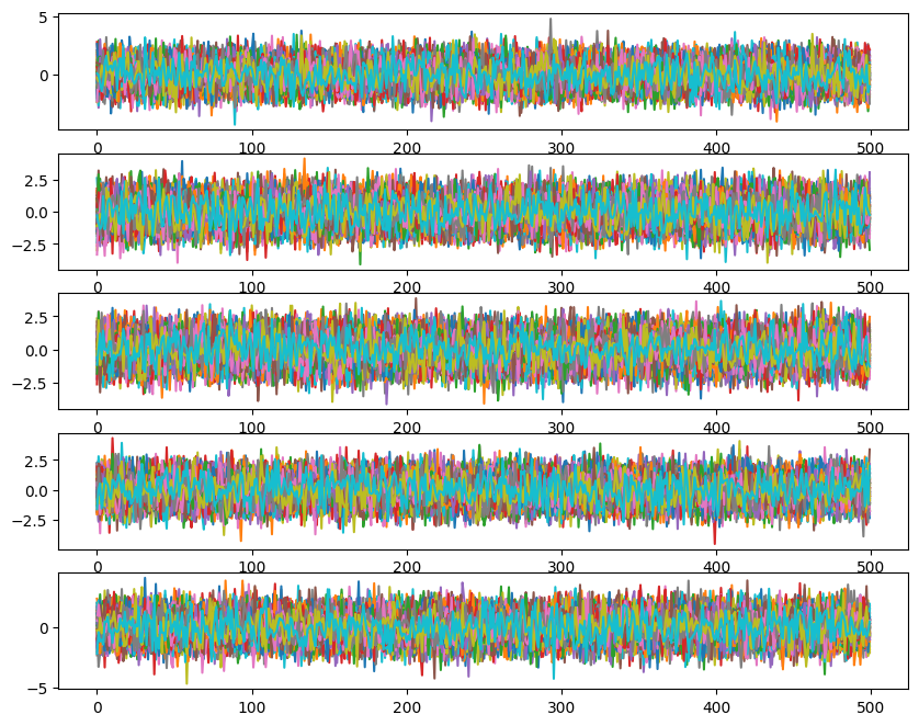
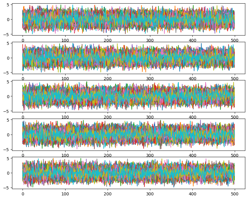
#### Chains
for temp in range(ntemps):
    fig, ax = plt.subplots(ndim, 1)
    fig.set_size_inches(10, 8)
    for i in range(ndim):
        for walk in range(nwalkers):
            ax[i].plot(ensemble_pt.get_chain()['model_0'][:, temp, walk, :, i])

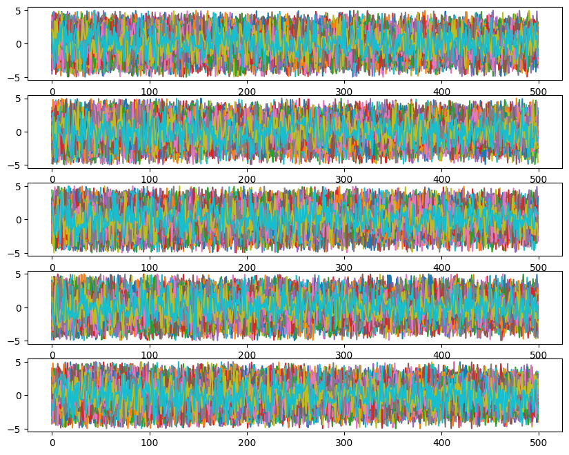
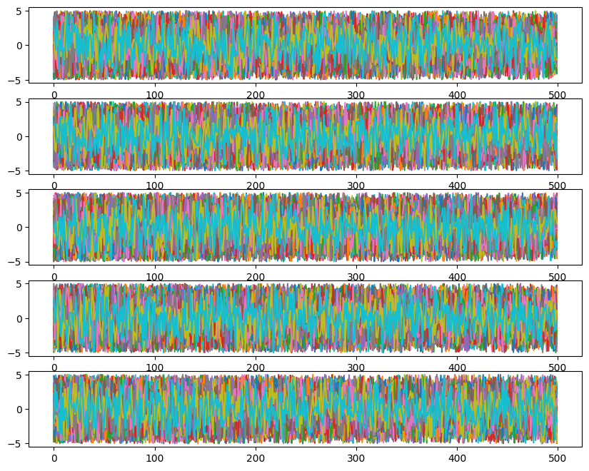
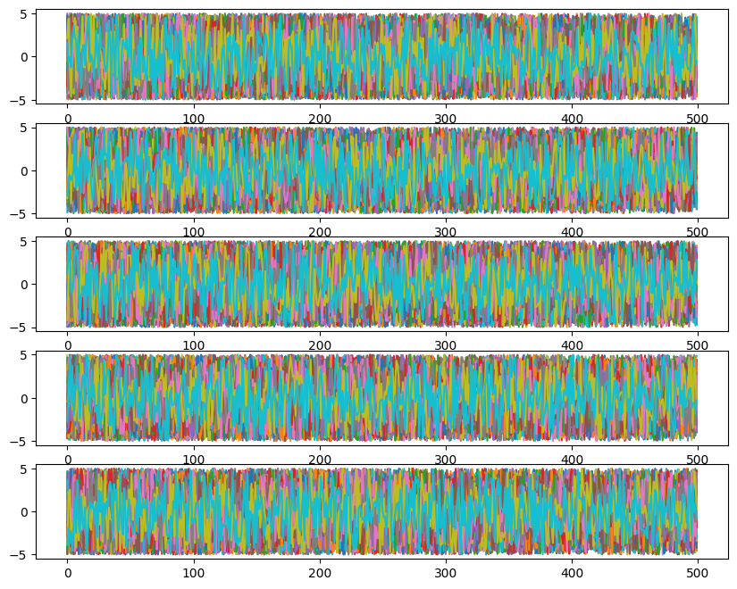
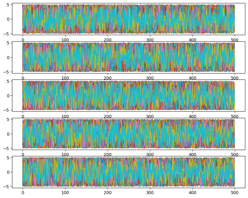
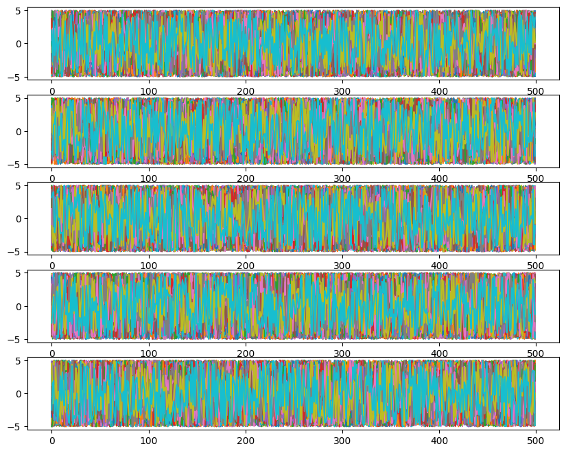
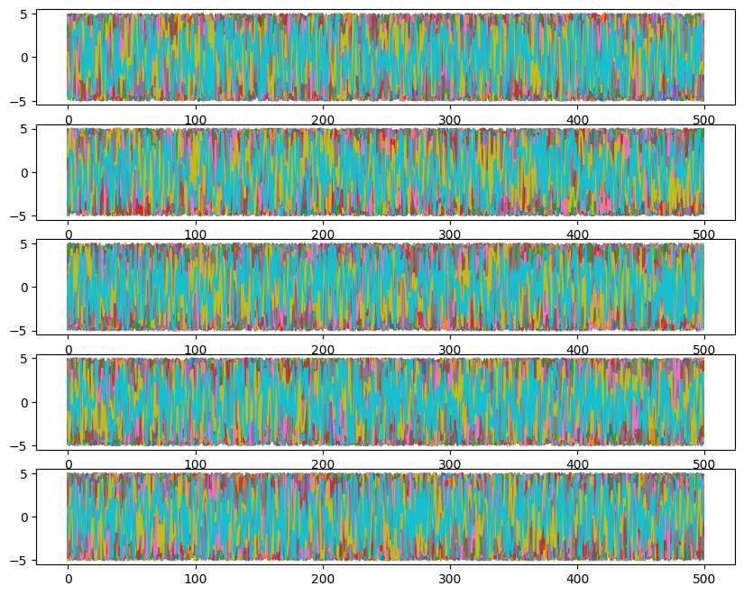
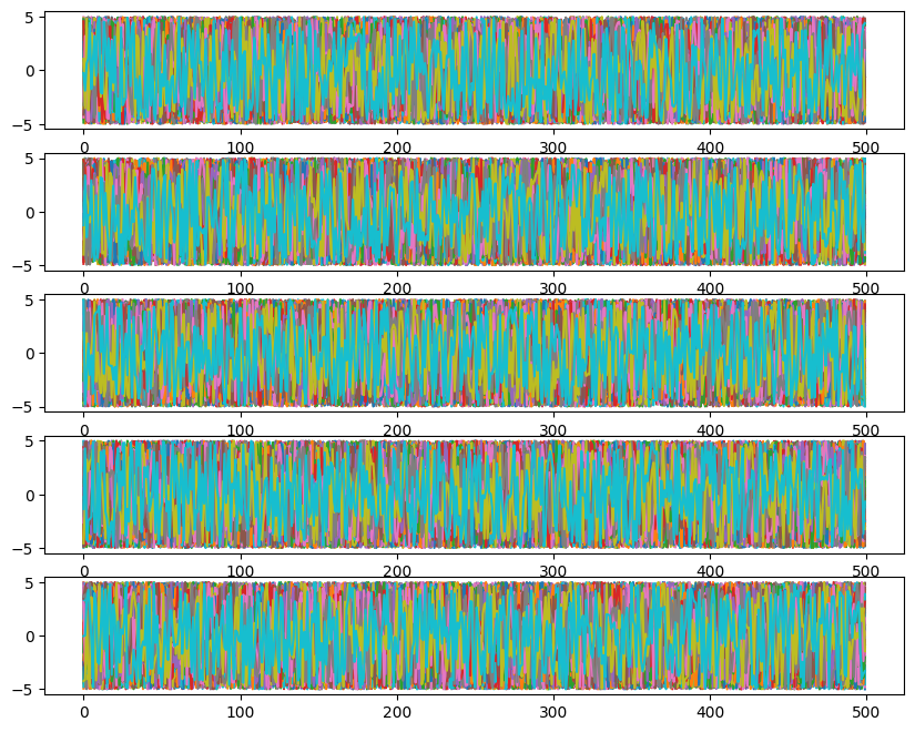
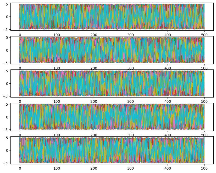
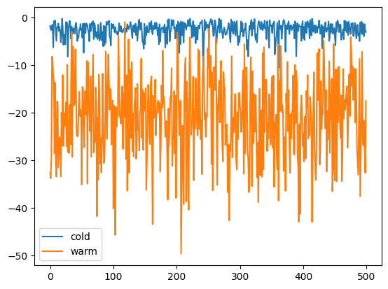
Likelihoods across temperatures:

ll = ensemble_pt.backend.get_log_like()
print(ll.shape)

# cold chain and highest temperature chain
plt.plot(ll[:, 0, 0], label="cold")
plt.plot(ll[:, -1, 0], label="warm")
plt.legend()

(500, 10, 100)

<matplotlib.legend.Legend at 0x138502ab0>

Add Reversible Jump MCMC (model count uncertainty)

We will now add to our sampler the ability to run with one branch, but a variable number of counts or leaves.

Here we are going to focus on the nested model case where we are just proposing changes in the model count. For more general review on Reversible Jump, see the Eryn paper and sources within.

In nested models, the acceptance probability for proposing to add a source is given by, \(\alpha_\text{nested}\),

\[\alpha_\text{nested} = \min\left(1, \frac{\mathcal{L}(\vec{\theta})_{k+1}}{\mathcal{L}(\vec{\theta})_{k}}\frac{p(\vec{\theta}_{+1})}{q(\vec{\theta}_{+1})}\right),\]

where there are \(k\) models to start, \(p(\vec{\theta}_{+1})\) is the prior probability of the added source only (the prior of the other sources cancels in the numerator and denominator), and \(q(\vec{\theta}_{+1})\) is the proposal distribution for the added source, \(\mathcal{L}(\vec{\theta})_k\) is the Likelihood for the position with \(k\) models, and \(\mathcal{L}(\vec{\theta})_{k+1}\) is the Likelihood for the position with \(k + 1\) models.

Reversible Jump proposals usually require specific implementations for each problem. We have one provided RJ proposal where we draw from the prior, which is the simplest and most generic reversible jump proposal for adding a nested model. In this case, the acceptance fraction just reduces to the Likelihood fraction.

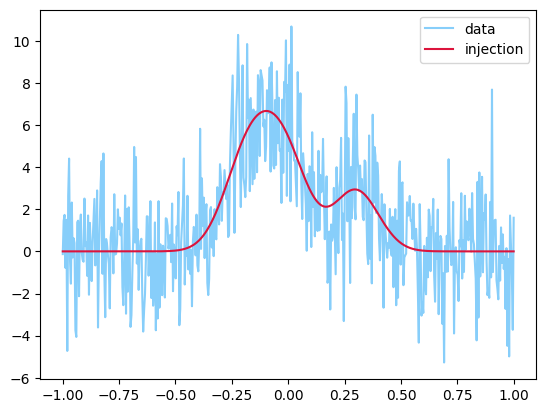
For this example, we will look at a set of 1D Gaussian pulses. We will inject a specific number, and then allow the sampler to determine the posterior probability on the model count, as well as the posterior on the parameters.

def gaussian_pulse(x, a, b, c):
    f_x = a * np.exp(-((x - b) ** 2) / (2 * c ** 2))
    return f_x

def combine_gaussians(t, params):
    template = np.zeros_like(t)
    for param in params:
        template += gaussian_pulse(t, *param)  # *params -> a, b, c
    return template

def log_like_fn_gauss_pulse(params, t, data, sigma):

    template = combine_gaussians(t, params)

    ll = -0.5 * np.sum(((template - data) / sigma) ** 2, axis=-1)
    return ll


nwalkers = 20
ntemps = 8
ndim = 3
nleaves_max = 8
nleaves_min = 0

branch_names = ["gauss"]

# define time stream
num = 500
t = np.linspace(-1, 1, num)

gauss_inj_params = [
    [3.3, -0.2, 0.1],
    [2.6, -0.1, 0.1],
    [3.4, 0.0, 0.1],
    [2.9, 0.3, 0.1],
]

# combine gaussians
injection = combine_gaussians(t, np.asarray(gauss_inj_params))

# set noise level
sigma = 2.0

# produce full data
y = injection + sigma * np.random.randn(len(injection))

plt.plot(t, y, label="data", color="lightskyblue")
plt.plot(t, injection, label="injection", color="crimson")
plt.legend()

<matplotlib.legend.Legend at 0x136e66450>

Setup our reversible-jump run

The first thing we do is setup our coords array. We have seen coords before. That array is the same but now nleaves_max > 1.

We also need to setup our inds arrays. inds is only needed when the dimensionality is changing (or more generally when not all leaves are used). inds is a boolean array with shape (ntemps, nwalkers, nleaves_max). It indicates which leaves are being used. This allows us to use the array structures while have a variable number of leaves per walker.

We are going to assume we have some knowledge of what is in the data, so we are going to start with 4 leaves for every walker. The burn-in will spread out the walkers both in terms of the parameters and in terms of the number of leaves per walker. Therefore, we are going to make the first four leaves in every walker True to indicate 4 sources. We are going to then put coordinates near each of the true Gaussians into coords.

coords = {"gauss": np.zeros((ntemps, nwalkers, nleaves_max, ndim))}

# this is the sigma for the multivariate Gaussian that sets starting points
# We need it to be very small to assume we are passed the search phase
# we will verify this is with likelihood calculations
sig1 = 0.0001

# setup initial walkers to be the correct count (it will spread out)
for nn in range(nleaves_max):
    if nn >= len(gauss_inj_params):
        # not going to add parameters for these unused leaves
        continue

    coords["gauss"][:, :, nn] = np.random.multivariate_normal(gauss_inj_params[nn], np.diag(np.ones(3) * sig1), size=(ntemps, nwalkers))

# make sure to start near the proper setup
inds = {"gauss": np.zeros((ntemps, nwalkers, nleaves_max), dtype=bool)}

# turn False -> True for any binary in the sampler
inds['gauss'][:, :, :len(gauss_inj_params)] = True

Priors are defined per model for a single model. It will take into account multiple models by summing the prior probability over the leaves.

# describes priors for all leaves independently
priors = {
    "gauss": {
        0: uniform_dist(2.5, 3.5),  # amplitude
        1: uniform_dist(t.min(), t.max()),  # mean
        2: uniform_dist(0.01, 0.21),  # sigma
    },
}

When reversible jump sampling is run, an RJ move (between model) is performed followed by an “in-model” move for each iteration of the sampler. “In-model” here means the model count is fixed, but the parameters are updated. We pass “in-model” moves to the sampler with the keyword argument moves. We pass RJ moves with the rj_moves keyword argument.

The stock proposal in Eryn is the stretch proposal. This proposal is only directly useful when the dimensionality is fixed. This will be discussed more below. When using reversible jump, we must choose our in-model proposal because the dimensionality is not fixed. Therefore, we choose to move our walkers with the most basic in-model move available: `eryn.moves.GaussianMove <https://mikekatz04.github.io/Eryn/html/user/moves.html#eryn.moves.GaussianMove>`__. For this move you can provide a covariance matrix that will be used in a multivariate Gaussian to propose new points that are centered on the current points (the means of the multivariate Gaussian will be the current point). This proposal is symmetric.

In this case, we are going to use the stock RJ proposal: `eryn.moves.PriorGenRj <https://mikekatz04.github.io/Eryn/html/user/moves.html#eryn.moves.DistributionGenerateRJ>`__. You can either pass this directly or you can set rj_moves to True (this is the default).

# for the Gaussian Move, will be explained later
factor = 0.00001
cov = {"gauss": np.diag(np.ones(ndim)) * factor}

moves = GaussianMove(cov)

We will now initialize the sampler by adding the branch, tempering, leaf, and move information.

ensemble = EnsembleSampler(
    nwalkers,
    ndim,
    log_like_fn_gauss_pulse,
    priors,
    args=[t, y, sigma],
    tempering_kwargs=dict(ntemps=ntemps),
    nbranches=len(branch_names),
    branch_names=branch_names,
    nleaves_max=nleaves_max,
    nleaves_min=nleaves_min,
    moves=moves,
    rj_moves=True,  # basic generation of new leaves from the prior
)

Now we will setup a State object and will use the Likelihood (compute_log_like) and prior functions (compute_log_prior) that are built into the sampler. The Likelihood function in the sampler will check the prior and only run walkers that exist entirely within the prior distribution. We can avoid redoing this computation by passing the prior as the logp kwarg to compute_log_like. The [0] at the end of the line is to grab the log Likelihood and leave behind any blobs.

log_prior = ensemble.compute_log_prior(coords, inds=inds)
log_like = ensemble.compute_log_like(coords, inds=inds, logp=log_prior)[0]

# make sure it is reasonably close to the maximum which this is
# will not be zero due to noise
print(log_like, log_prior)

# setup starting state
state = State(coords, log_like=log_like, log_prior=log_prior, inds=inds)

[[-267.48857258 -273.13358068 -272.04356318 -273.41959181 -269.65159976
  -273.45581292 -269.0534354  -269.21480317 -270.17335397 -268.79114293
  -267.97593006 -269.76118281 -268.97477874 -268.96915067 -267.44497304
  -268.55232307 -268.69079155 -269.13611008 -266.317588   -268.19035794]
 [-267.89498107 -271.07519263 -271.01364247 -269.87074404 -271.04982746
  -273.10216287 -270.47561552 -268.73825004 -268.55984235 -267.59669384
  -269.1644275  -268.17686823 -269.5530668  -266.38471516 -270.13810357
  -268.4965744  -271.16336376 -268.37273575 -269.78843561 -266.07926996]
 [-266.65635127 -268.4524668  -269.58696913 -269.88671242 -266.37498437
  -266.44936502 -266.4546787  -272.25432486 -269.746439   -273.53395912
  -268.78432036 -268.09641939 -269.51993913 -270.03690593 -268.47293353
  -270.13166208 -267.3654575  -272.4533991  -267.76589766 -268.67119754]
 [-268.70301053 -268.05419472 -266.85429247 -268.34706671 -272.61170665
  -270.35744037 -267.49130951 -266.41191836 -275.34555909 -267.63796847
  -268.91668611 -268.75395295 -265.89682062 -265.78621765 -269.99614319
  -266.0744601  -267.66910539 -271.02551726 -268.96820568 -272.10089077]
 [-269.36015159 -267.91718124 -266.58033431 -270.98339743 -271.82208208
  -271.73487149 -269.30751278 -269.16895186 -266.30161    -272.80287899
  -269.03261838 -269.48740534 -270.6325905  -267.60035469 -268.2688322
  -274.62821662 -266.26778016 -267.04032577 -270.28884496 -269.45920218]
 [-267.25519775 -267.62892664 -272.26285005 -267.00766373 -269.57983127
  -274.27398717 -268.46784025 -271.09344272 -271.24621424 -267.80982016
  -273.18463057 -268.36312445 -270.59373649 -270.557759   -271.87911261
  -266.02454376 -266.93381068 -278.98378996 -269.83416176 -268.05726244]
 [-267.02005355 -268.09999743 -269.06119558 -268.00971489 -268.12141711
  -268.14986569 -268.14312728 -267.72178265 -271.78486633 -270.33369975
  -268.45148378 -269.87881376 -268.72205688 -270.82850441 -267.57604611
  -266.79122124 -267.35162949 -267.59266883 -267.114322   -270.56048742]
 [-267.67914435 -266.02251242 -266.32624169 -269.16921554 -268.73743926
  -274.21583965 -269.74454528 -269.21673563 -268.68519371 -266.60927311
  -270.20377505 -267.99209023 -269.13139001 -268.27709924 -265.67000643
  -274.6973296  -269.6495672  -269.3549933  -269.01571009 -267.5950623 ]] [[3.66516293 3.66516293 3.66516293 3.66516293 3.66516293 3.66516293
  3.66516293 3.66516293 3.66516293 3.66516293 3.66516293 3.66516293
  3.66516293 3.66516293 3.66516293 3.66516293 3.66516293 3.66516293
  3.66516293 3.66516293]
 [3.66516293 3.66516293 3.66516293 3.66516293 3.66516293 3.66516293
  3.66516293 3.66516293 3.66516293 3.66516293 3.66516293 3.66516293
  3.66516293 3.66516293 3.66516293 3.66516293 3.66516293 3.66516293
  3.66516293 3.66516293]
 [3.66516293 3.66516293 3.66516293 3.66516293 3.66516293 3.66516293
  3.66516293 3.66516293 3.66516293 3.66516293 3.66516293 3.66516293
  3.66516293 3.66516293 3.66516293 3.66516293 3.66516293 3.66516293
  3.66516293 3.66516293]
 [3.66516293 3.66516293 3.66516293 3.66516293 3.66516293 3.66516293
  3.66516293 3.66516293 3.66516293 3.66516293 3.66516293 3.66516293
  3.66516293 3.66516293 3.66516293 3.66516293 3.66516293 3.66516293
  3.66516293 3.66516293]
 [3.66516293 3.66516293 3.66516293 3.66516293 3.66516293 3.66516293
  3.66516293 3.66516293 3.66516293 3.66516293 3.66516293 3.66516293
  3.66516293 3.66516293 3.66516293 3.66516293 3.66516293 3.66516293
  3.66516293 3.66516293]
 [3.66516293 3.66516293 3.66516293 3.66516293 3.66516293 3.66516293
  3.66516293 3.66516293 3.66516293 3.66516293 3.66516293 3.66516293
  3.66516293 3.66516293 3.66516293 3.66516293 3.66516293 3.66516293
  3.66516293 3.66516293]
 [3.66516293 3.66516293 3.66516293 3.66516293 3.66516293 3.66516293
  3.66516293 3.66516293 3.66516293 3.66516293 3.66516293 3.66516293
  3.66516293 3.66516293 3.66516293 3.66516293 3.66516293 3.66516293
  3.66516293 3.66516293]
 [3.66516293 3.66516293 3.66516293 3.66516293 3.66516293 3.66516293
  3.66516293 3.66516293 3.66516293 3.66516293 3.66516293 3.66516293
  3.66516293 3.66516293 3.66516293 3.66516293 3.66516293 3.66516293
  3.66516293 3.66516293]]

Run the sampler

nsteps = 2000
last_sample = ensemble.run_mcmc(state, nsteps, burn=1000, progress=True, thin_by=1)

100%|███████████████████████████████████████| 1000/1000 [00:36<00:00, 27.08it/s]
100%|███████████████████████████████████████| 2000/2000 [01:13<00:00, 27.27it/s]

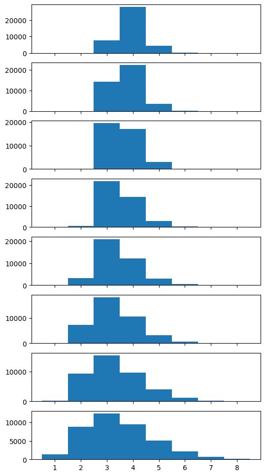
Let’s look at the last sample in terms of the nleaves array.

last_sample.branches["gauss"].nleaves

array([[4, 4, 3, 4, 4, 3, 4, 4, 4, 4, 3, 4, 4, 4, 4, 3, 4, 3, 5, 3],
       [3, 4, 3, 3, 4, 4, 4, 3, 4, 3, 3, 4, 3, 3, 4, 4, 4, 4, 4, 4],
       [4, 4, 3, 3, 3, 3, 3, 4, 4, 4, 4, 4, 5, 3, 5, 3, 4, 5, 4, 3],
       [3, 4, 3, 3, 3, 3, 3, 4, 3, 3, 4, 5, 3, 4, 4, 3, 3, 3, 4, 4],
       [3, 3, 2, 3, 4, 5, 5, 5, 4, 6, 4, 3, 5, 3, 3, 5, 3, 4, 4, 5],
       [4, 4, 3, 3, 2, 2, 2, 4, 3, 3, 3, 3, 3, 2, 5, 3, 2, 3, 3, 4],
       [3, 3, 2, 2, 4, 4, 2, 3, 4, 2, 2, 4, 3, 2, 3, 6, 3, 2, 2, 2],
       [2, 5, 5, 3, 4, 3, 4, 4, 7, 2, 3, 2, 5, 5, 3, 3, 4, 2, 2, 3]])

print(f'max ll: {ensemble.get_log_like().max()}')

nleaves = ensemble.get_nleaves()['gauss']
bns = (
    np.arange(1, nleaves_max + 2) - 0.5
)  # Just to make it pretty and center the bins

fig, ax = plt.subplots(ntemps, 1, sharex=True)
fig.set_size_inches(6, 12)
for temp, ax_t in enumerate(ax):
    ax_t.hist(nleaves[:, temp].flatten(), bins=bns)

max ll: -261.2302411532098

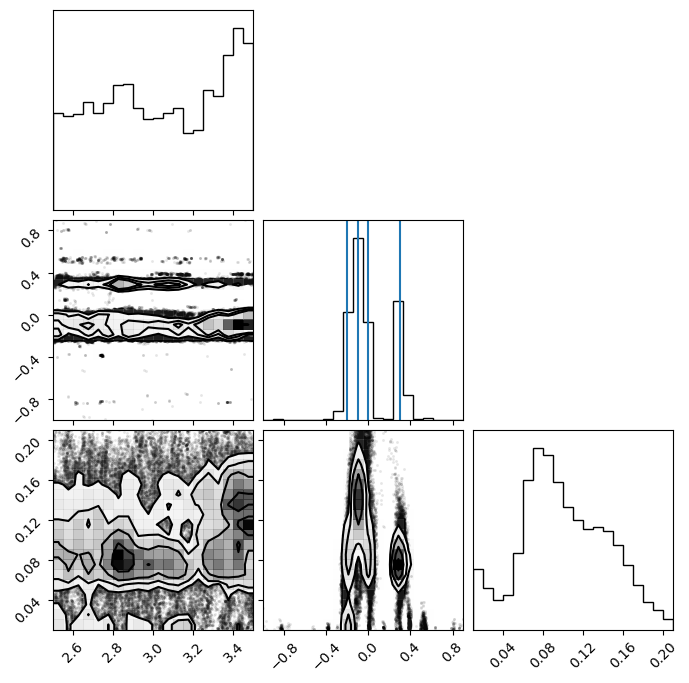
To get the samples, we need remove any sources that were not used. We can combine coords and inds or we can remove anywhere where the backend returns Nan. Backends store Nan for the coordinates that belong to sources that are not currently used (inds == False).

samples = ensemble.get_chain()['gauss'][:, 0].reshape(-1, ndim)

# same as ensemble.get_chain()['gauss'][ensemble.get_inds()['gauss']]
samples = samples[~np.isnan(samples[:, 0])]

means = np.asarray(gauss_inj_params)[:, 1]

fig = corner.corner(samples)

ax = fig.axes

for mean in means:
    ax[4].axvline(mean)

Add multiple branches

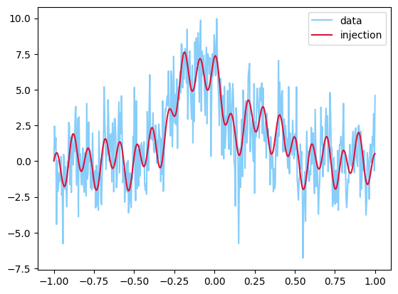
Now we will add another model to our reversible jump problem. We will add a sine wave model.

def gaussian_pulse(x, a, b, c):
    f_x = a * np.exp(-((x - b) ** 2) / (2 * c ** 2))
    return f_x

def combine_gaussians(t, params):
    template = np.zeros_like(t)
    for param in params:
        template += gaussian_pulse(t, *param)  # *params -> a, b, c
    return template

def sine(x, a, b, c):
    f_x = a * np.sin(2 * np.pi * b * x + c)
    return f_x

def combine_sine(t, params):
    template = np.zeros_like(t)
    for param in params:
        template += sine(t, *param)  # *params -> a, b, c
    return template

def log_like_fn_gauss_and_sine(params_both, t, data, sigma):

    params_gauss, params_sine = params_both
    template = np.zeros_like(t)

    if params_gauss is not None:
        template += combine_gaussians(t, params_gauss)

    if params_sine is not None:
        template += combine_sine(t, params_sine)

    ll = -0.5 * np.sum(((template - data) / sigma) ** 2, axis=-1)
    return ll


nwalkers = 20
ntemps = 8
ndims = {"gauss": 3, "sine": 3}
nleaves_max = {"gauss": 8, "sine": 4}
nleaves_min = {"gauss": 0, "sine": 0}

branch_names = ["gauss", "sine"]

# define time stream
num = 500
t = np.linspace(-1, 1, num)

gauss_inj_params = [
    [3.3, -0.2, 0.1],
    [2.6, -0.1, 0.1],
    [3.4, 0.0, 0.1],
    [2.9, 0.3, 0.1],
]

sine_inj_params = [
    [1.3, 10.1, 1.0],
    [0.8, 4.6, 1.2],
]

# combine gaussians
injection = combine_gaussians(t, np.asarray(gauss_inj_params))
injection += combine_sine(t, np.asarray(sine_inj_params))

# set noise level
sigma = 2.0

# produce full data
y = injection + sigma * np.random.randn(len(injection))

plt.plot(t, y, label="data", color="lightskyblue")
plt.plot(t, injection, label="injection", color="crimson")
plt.legend()

<matplotlib.legend.Legend at 0x135c54e60>

coords and inds

coords = {
    "gauss": np.zeros((ntemps, nwalkers, nleaves_max["gauss"], ndims["gauss"])),
    "sine": np.zeros((ntemps, nwalkers, nleaves_max["sine"], ndims["sine"]))
}

# make sure to start near the proper setup
inds = {
    "gauss": np.zeros((ntemps, nwalkers, nleaves_max["gauss"]), dtype=bool),
    "sine": np.zeros((ntemps, nwalkers, nleaves_max["sine"]), dtype=bool)
}


# this is the sigma for the multivariate Gaussian that sets starting points
# We need it to be very small to assume we are passed the search phase
# we will verify this is with likelihood calculations
sig1 = 0.0001

# setup initial walkers to be the correct count (it will spread out)
# start with gaussians
for nn in range(nleaves_max["gauss"]):
    if nn >= len(gauss_inj_params):
        # not going to add parameters for these unused leaves
        continue
    coords["gauss"][:, :, nn] = np.random.multivariate_normal(gauss_inj_params[nn], np.diag(np.ones(3) * sig1), size=(ntemps, nwalkers))
    inds["gauss"][:, :, nn] = True

# next do sine waves
for nn in range(nleaves_max["sine"]):
    if nn >= len(sine_inj_params):
        # not going to add parameters for these unused leaves
        continue
    coords["sine"][:, :, nn] = np.random.multivariate_normal(sine_inj_params[nn], np.diag(np.ones(3) * sig1), size=(ntemps, nwalkers))
    inds["sine"][:, :, nn] = True

Priors are defined per model for a single model. It will take into account multiple models by summing the prior probability over the leaves.

# describes priors for all leaves independently
priors = {
    "gauss": {
        0: uniform_dist(2.5, 3.5),  # amplitude
        1: uniform_dist(t.min(), t.max()),  # mean
        2: uniform_dist(0.01, 0.21),  # sigma
    },
    "sine": {
        0: uniform_dist(0.5, 1.5),  # amplitude
        1: uniform_dist(1., 20.),  # mean
        2: uniform_dist(0.0, 2 * np.pi),  # sigma
    },
}

You can add multiple covariance matrices. One for each branch. We will keep it the same for simplicity.

# for the Gaussian Move, will be explained later
factor = 0.00001
cov = {
    "gauss": np.diag(np.ones(ndims["gauss"])) * factor,
    "sine": np.diag(np.ones(ndims["sine"])) * factor
}

moves = GaussianMove(cov)

We will now initialize the sampler by adding the branch, tempering, leaf, and move information.

ensemble = EnsembleSampler(
    nwalkers,
    ndims,
    log_like_fn_gauss_and_sine,
    priors,
    args=[t, y, sigma],
    tempering_kwargs=dict(ntemps=ntemps),
    nbranches=len(branch_names),
    branch_names=branch_names,
    nleaves_max=nleaves_max,
    nleaves_min=nleaves_min,
    moves=moves,
    rj_moves=True,  # basic generation of new leaves from the prior
)

Prior, Likelihood, and initial state.

log_prior = ensemble.compute_log_prior(coords, inds=inds)
log_like = ensemble.compute_log_like(coords, inds=inds, logp=log_prior)[0]

# make sure it is reasonably close to the maximum which this is
# will not be zero due to noise
print(log_like, log_prior)

# setup starting state
state = State(coords, log_like=log_like, log_prior=log_prior, inds=inds)

[[-229.18441391 -233.51872418 -231.94801463 -235.4050852  -226.670966
  -232.71483467 -229.99148863 -232.40535129 -229.22825659 -230.16495346
  -228.29127145 -228.74374649 -226.49117628 -231.25563257 -228.862688
  -227.44352935 -234.67849744 -231.49859258 -230.65579296 -231.81069992]
 [-227.81377327 -230.13945878 -229.41654888 -227.94783414 -229.31522738
  -229.81615798 -229.78817956 -227.80534798 -231.90524192 -228.65212536
  -230.79128554 -227.40049869 -231.24527916 -234.05736224 -238.63570222
  -231.43650992 -235.70464801 -231.34328242 -228.12956141 -229.26914673]
 [-230.26442866 -226.47503056 -231.56851138 -229.37430551 -228.93271986
  -230.38850202 -232.53092761 -235.03556521 -231.54049548 -229.99913862
  -232.53777598 -228.16530309 -230.35808751 -227.22674918 -226.15827365
  -236.00134375 -235.68397539 -226.24369726 -231.68966882 -227.59454795]
 [-231.95358162 -228.82307944 -235.14353803 -229.14890501 -232.15227879
  -228.64013278 -228.89132475 -234.37202006 -227.71900568 -227.70720334
  -230.98768038 -232.11278035 -228.33877408 -241.12287975 -232.40874977
  -230.84468334 -233.2095918  -230.99834849 -231.10304391 -227.32449253]
 [-229.1865482  -230.04713397 -232.82592779 -229.51721312 -226.95258359
  -230.80694449 -228.14420069 -230.90414617 -233.609932   -228.10522529
  -230.85522437 -229.68349989 -230.10665679 -229.19997595 -234.44616622
  -228.85330281 -234.27875953 -233.58673313 -228.10932674 -234.29296705]
 [-233.95788218 -228.0866977  -233.30264265 -228.82346604 -229.72494204
  -234.28165905 -238.15989341 -234.29506362 -230.50970622 -230.71630602
  -230.12739788 -231.63811447 -233.83828594 -229.67742849 -228.6620161
  -238.63551634 -228.32572285 -228.24280784 -234.38914285 -228.14806505]
 [-229.23356207 -234.67103428 -237.90881138 -233.83466125 -231.34757217
  -229.55405955 -231.77788649 -232.20798465 -229.09701881 -233.44980698
  -226.98678903 -231.26528224 -229.38754856 -231.85794747 -231.22487614
  -234.95102489 -232.95030022 -228.22226315 -231.56264544 -229.59721156]
 [-231.90934207 -234.26628503 -229.59759858 -226.18117692 -228.3581854
  -227.89490619 -232.35931607 -227.58448115 -237.42531875 -233.79614919
  -229.43853536 -232.59733154 -228.00377491 -228.39675954 -233.79924613
  -226.68628461 -228.18445055 -229.21994604 -229.56782994 -230.51977065]] [[-5.89946916 -5.89946916 -5.89946916 -5.89946916 -5.89946916 -5.89946916
  -5.89946916 -5.89946916 -5.89946916 -5.89946916 -5.89946916 -5.89946916
  -5.89946916 -5.89946916 -5.89946916 -5.89946916 -5.89946916 -5.89946916
  -5.89946916 -5.89946916]
 [-5.89946916 -5.89946916 -5.89946916 -5.89946916 -5.89946916 -5.89946916
  -5.89946916 -5.89946916 -5.89946916 -5.89946916 -5.89946916 -5.89946916
  -5.89946916 -5.89946916 -5.89946916 -5.89946916 -5.89946916 -5.89946916
  -5.89946916 -5.89946916]
 [-5.89946916 -5.89946916 -5.89946916 -5.89946916 -5.89946916 -5.89946916
  -5.89946916 -5.89946916 -5.89946916 -5.89946916 -5.89946916 -5.89946916
  -5.89946916 -5.89946916 -5.89946916 -5.89946916 -5.89946916 -5.89946916
  -5.89946916 -5.89946916]
 [-5.89946916 -5.89946916 -5.89946916 -5.89946916 -5.89946916 -5.89946916
  -5.89946916 -5.89946916 -5.89946916 -5.89946916 -5.89946916 -5.89946916
  -5.89946916 -5.89946916 -5.89946916 -5.89946916 -5.89946916 -5.89946916
  -5.89946916 -5.89946916]
 [-5.89946916 -5.89946916 -5.89946916 -5.89946916 -5.89946916 -5.89946916
  -5.89946916 -5.89946916 -5.89946916 -5.89946916 -5.89946916 -5.89946916
  -5.89946916 -5.89946916 -5.89946916 -5.89946916 -5.89946916 -5.89946916
  -5.89946916 -5.89946916]
 [-5.89946916 -5.89946916 -5.89946916 -5.89946916 -5.89946916 -5.89946916
  -5.89946916 -5.89946916 -5.89946916 -5.89946916 -5.89946916 -5.89946916
  -5.89946916 -5.89946916 -5.89946916 -5.89946916 -5.89946916 -5.89946916
  -5.89946916 -5.89946916]
 [-5.89946916 -5.89946916 -5.89946916 -5.89946916 -5.89946916 -5.89946916
  -5.89946916 -5.89946916 -5.89946916 -5.89946916 -5.89946916 -5.89946916
  -5.89946916 -5.89946916 -5.89946916 -5.89946916 -5.89946916 -5.89946916
  -5.89946916 -5.89946916]
 [-5.89946916 -5.89946916 -5.89946916 -5.89946916 -5.89946916 -5.89946916
  -5.89946916 -5.89946916 -5.89946916 -5.89946916 -5.89946916 -5.89946916
  -5.89946916 -5.89946916 -5.89946916 -5.89946916 -5.89946916 -5.89946916
  -5.89946916 -5.89946916]]

Run the sampler

state.branches

{'gauss': <eryn.state.Branch at 0x135c56d20>,
 'sine': <eryn.state.Branch at 0x135c576b0>}

nsteps = 5000
last_sample = ensemble.run_mcmc(state, nsteps, burn=1000, progress=True, thin_by=1)

100%|███████████████████████████████████████| 1000/1000 [00:55<00:00, 18.07it/s]
100%|███████████████████████████████████████| 5000/5000 [04:22<00:00, 19.08it/s]

Let’s look at the last sample in terms of the nleaves array for both branches in the cold chain.

np.array([last_sample.branches["gauss"].nleaves[0], last_sample.branches["sine"].nleaves[0]]).T

array([[4, 2],
       [4, 2],
       [4, 2],
       [4, 2],
       [4, 2],
       [4, 2],
       [4, 2],
       [4, 2],
       [4, 2],
       [3, 3],
       [4, 2],
       [4, 2],
       [4, 2],
       [4, 2],
       [4, 2],
       [4, 2],
       [4, 2],
       [4, 2],
       [4, 2],
       [4, 2]])

print(f'max ll: {ensemble.get_log_like().max()}')

nleaves_gauss = ensemble.get_nleaves()['gauss']
nleaves_sine = ensemble.get_nleaves()['sine']
bns = (
    np.arange(1, nleaves_max["gauss"] + 2) - 0.5
)  # Just to make it pretty and center the bins

fig, ax = plt.subplots(ntemps, 1, sharex=True)
fig.set_size_inches(6, 12)
for temp, ax_t in enumerate(ax):
    ax_t.hist(nleaves_gauss[:, temp].flatten(), bins=bns, histtype="step", label="gauss")
    ax_t.hist(nleaves_sine[:, temp].flatten(), bins=bns, histtype="step", label="sine")
ax[0].legend()

max ll: -218.81128464457333

<matplotlib.legend.Legend at 0x138ba86b0>

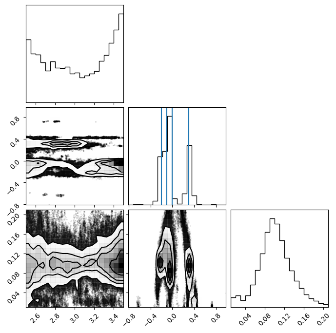
To get the samples, we need remove any sources that were not used. We can combine coords and inds or we can remove anywhere where the backend returns Nan. Backends store Nan for the coordinates that belong to binaries that are not currently used (inds == False).

samples = ensemble.get_chain()['gauss'][:, 0].reshape(-1, ndim)

# same as ensemble.get_chain()['gauss'][ensemble.get_inds()['gauss']]
samples = samples[~np.isnan(samples[:, 0])]

means = np.asarray(gauss_inj_params)[:, 1]

fig = corner.corner(samples)

ax = fig.axes

for mean in means:
    ax[4].axvline(mean)

Moves

Moves are generally implemented with the same three-tier structure that originated in emcee. For full documentation on all available moves, as well as class inheritance information, see the Move documentation. For implementing customized moves, we recommend using the documentation as well as the various source codes for guidance.

from eryn.moves:

• Base Move Class (Move)

• Move Guide (MHMove, RedBlueMove, ReversibleJumpMove, GroupMove)

• Proposal Class (e.g. StretchMove, GaussianMove, GroupStretchMove, DistributionGenerateRJ).

The eryn.moves.Move class is a base class for all moves. It houses the tempering information class (eryn.moves.TemperatureControl), as well as other information and methods that apply universally to most or all moves.

The Move Guides provide the overall computation of the different types of moves depending on how they are executed. Their main purpose is to implement the propose(model, state) function. They all return a tuple of updated State objects and an boolean array of accepted information.

• MHMove: These moves move all walkers simultaneously as an in-model move without using any information from current walkers.

• RedBlueMove: These moves move half of the distribution first and then the other half. This allows for parallel updates of moves that use current walkers for move information. This strategy was first proposed in emcee.

• GroupMoves: These moves can move all walkers at once. They are similar to the RedBlueMove but instead of using current walkers, they use a stationary distribution of walkers that does not change each proposal. Ideally, the distribution changes infrequently.

• ReversibleJumpMove: This class guides Reversible Jump MCMC moves. The key difference to the other moves is that the inds array changes adjust the model type and/or count. It is very common in Reversible Jump settings to have to implemement a specific RJ proposal. One of the main goals of Eryn is to distill this process down to this step and keep the rest of the sampler apparatus the same between projects.

Example diagonal covariance move

When implemented a move at the Proposal Class layer, you only need to implement the get_proposal method. Look at the call signature from the chosen Move Guide. You can obviously implement more than that.

from eryn.moves import MHMove

class NonScaledDiagonalGaussianMove(MHMove):
    def __init__(self, cov_all, *args, **kwargs):

        # checks
        for branch_name, cov in cov_all.items():
            assert isinstance(cov, np.ndarray) and cov.ndim == 1

        # store for later
        self.cov = cov_all

        # initialize any parent class information
        super(NonScaledDiagonalGaussianMove, self).__init__(*args, **kwargs)

    def get_proposal(self, branches_coords, random, branches_inds=None, **kwargs):

        assert branches_inds is not None
        new_points = {}
        for name, cov in self.cov.items():
            assert name in branches_coords
            coords = branches_coords[name]
            inds = branches_inds[name]

            ntemps, nwalkers, nleaves_max, ndim = coords.shape

            # generate sigma from normal distribution
            sigma = random.randn(ntemps, nwalkers)

            tmp = np.zeros_like(coords)

            tmp = coords + sigma[:, :, None, None] * cov[None, None, None, :]
            # symmetric
            new_points[name] = np.zeros_like(coords)

            # this is not necessary as the inds will remove there changes in the parent class
            # but I put it here to indicate to think about it
            new_points[name][inds] = tmp[inds]

        # symmetric
        factors = np.zeros((ntemps, nwalkers))

        return new_points, factors

Gibbs Sampling

There is a very useful setup for Gibbs sampling of parameters in Eryn. To use this feature, you can pass information as the gibbs_sampling_setup keyword argument to the chosen Move class. It is handled by the base eryn.moves.Move class so it is a feature of all proposals.

Gibbs sampling allows the user to sample over a specific set of models or parameters to improve sampling efficiency. For example, sampling in a 100-parameter space may be inefficient, but sampling in 10-dimensional sub-spaces consecutively may be more efficient by increasing the acceptance fraction.

The documentation for the gibbs_sampling_setup parameter reads as follows:

gibbs_sampling_setup (str, tuple, dict, or list, optional) – This sets the Gibbs Sampling setup if desired. The Gibbs sampling setup is completely customizable down to the leaf and parameters. All of the separate Gibbs sampling splits will be run within 1 call to this proposal. If None, run all branches and all parameters. If str, run all parameters within the branch given as the string. To enter a branch with a specific set of parameters, you can provide a 2-tuple with the first entry as the branch name and the second entry as a 2D boolean array of shape (nleaves_max, ndim) that indicates which leaves and/or parameters you want to run. None can also be entered in the second entry if all parameters are to be run. A dictionary is also possible with keys as branch names and values as the same 2D boolean array of shape (nleaves_max, ndim) that indicates which leaves and/or parameters you want to run. None can also be entered in the value of the dictionary if all parameters are to be run. If multiple keys are provided in the dictionary, those branches will be run simultaneously in the proposal as one iteration of the proposing loop. The final option is a list. This is how you make sure to run all the Gibbs splits. Each entry of the list can be a string, 2-tuple, or dictionary as described above. The list controls the order in which all of these splits are run. (default: None)

In the following example, we will use Gibbs sampling to run the same multimodel case as above with the sine waves and Gaussian pulses. However, in the example above, for each proposal, both in-model and between-model, all parameters/leaves were updated simultaneously. This means for the in-model step, all parameters for both models were updated simultaneously. In the between-model or RJ step, changes to the leaf counts were also proposed simultaneously for both models. In simple cases, the may be okay.

Here we will fix the model count of the sine waves to the true value in order to use the stretch proposal on that model. We will still sample over Gaussian pulses with an uncertain model count. We will choose for the sake of example to sample leaf by leaf over the first 2 parameters of the sine wave and then the last one. For the Gaussians, we will sample all the parameters together, but leaf by leaf.

We will also use the CombineMove to make sure these all happen one after another.

nwalkers = 20
ntemps = 8
ndims = {"gauss": 3, "sine": 3}
nleaves_max = {"gauss": 8, "sine": 2} # same min and max means no changing
nleaves_min = {"gauss": 0, "sine": 2}

branch_names = ["gauss", "sine"]

# define time stream
num = 500
t = np.linspace(-1, 1, num)

gauss_inj_params = [
    [3.3, -0.2, 0.1],
    [2.6, -0.1, 0.1],
    [3.4, 0.0, 0.1],
    [2.9, 0.3, 0.1],
]

sine_inj_params = [
    [1.3, 10.1, 1.0],
    [0.8, 4.6, 1.2],
]

# combine gaussians
injection = combine_gaussians(t, np.asarray(gauss_inj_params))
injection += combine_sine(t, np.asarray(sine_inj_params))

# set noise level
sigma = 2.0

# produce full data
y = injection + sigma * np.random.randn(len(injection))


coords = {
    "gauss": np.zeros((ntemps, nwalkers, nleaves_max["gauss"], ndims["gauss"])),
    "sine": np.zeros((ntemps, nwalkers, nleaves_max["sine"], ndims["sine"]))
}

# make sure to start near the proper setup
inds = {
    "gauss": np.zeros((ntemps, nwalkers, nleaves_max["gauss"]), dtype=bool),
    "sine": np.ones((ntemps, nwalkers, nleaves_max["sine"]), dtype=bool)
}


# this is the sigma for the multivariate Gaussian that sets starting points
# We need it to be very small to assume we are passed the search phase
# we will verify this is with likelihood calculations
sig1 = 0.0001

# setup initial walkers to be the correct count (it will spread out)
# start with gaussians
for nn in range(nleaves_max["gauss"]):
    if nn >= len(gauss_inj_params):
        # not going to add parameters for these unused leaves
        continue
    coords["gauss"][:, :, nn] = np.random.multivariate_normal(gauss_inj_params[nn], np.diag(np.ones(3) * sig1), size=(ntemps, nwalkers))
    inds["gauss"][:, :, nn] = True

# next do sine waves
for nn in range(nleaves_max["sine"]):
    if nn >= len(sine_inj_params):
        # not going to add parameters for these unused leaves
        continue
    coords["sine"][:, :, nn] = np.random.multivariate_normal(sine_inj_params[nn], np.diag(np.ones(3) * sig1), size=(ntemps, nwalkers))
    # inds["sine"][:, :, nn] = True  # already True


# describes priors for all leaves independently
priors = {
    "gauss": {
        0: uniform_dist(2.5, 3.5),  # amplitude
        1: uniform_dist(t.min(), t.max()),  # mean
        2: uniform_dist(0.01, 0.21),  # sigma
    },
    "sine": {
        0: uniform_dist(0.5, 1.5),  # amplitude
        1: uniform_dist(1., 20.),  # mean
        2: uniform_dist(0.0, 2 * np.pi),  # sigma
    },
}

# for the Gaussian Move
factor = 0.00001
cov = {
    "gauss": np.diag(np.ones(ndims["gauss"])) * factor,
}

# pass boolean array of shape (nleaves_max["gauss"], ndims["gauss"])
gibbs_sampling_gauss = [
    ("gauss", np.zeros((nleaves_max["gauss"], ndims["gauss"]), dtype=bool))
    for _ in range(nleaves_max["gauss"])
]

for i in range(nleaves_max["gauss"]):
    gibbs_sampling_gauss[i][-1][i] = True

gauss_move = GaussianMove(cov, gibbs_sampling_setup=gibbs_sampling_gauss)

print("gauss gibbs setup:", gibbs_sampling_gauss)

gibbs_sampling_sine = [
    ("sine", np.zeros((nleaves_max["sine"], ndims["sine"]), dtype=bool))
    for _ in range(2 * nleaves_max["sine"])
]
for i in range(nleaves_max["sine"]):
    for j in range(2):
        if j == 0:
            gibbs_sampling_sine[2 * i + j][-1][i, :2] = True
        else:
            gibbs_sampling_sine[2 * i + j][-1][i, 2:] = True

print("sine gibbs setup:", gibbs_sampling_sine)

sine_move = StretchMove(live_dangerously=True, gibbs_sampling_setup=gibbs_sampling_sine)

move = CombineMove([gauss_move, sine_move])

ensemble = EnsembleSampler(
    nwalkers,
    ndims,
    log_like_fn_gauss_and_sine,
    priors,
    args=[t, y, sigma],
    tempering_kwargs=dict(ntemps=ntemps),
    nbranches=len(branch_names),
    branch_names=branch_names,
    nleaves_max=nleaves_max,
    nleaves_min=nleaves_min,
    moves=move,
    rj_moves=True,  # basic generation of new leaves from the prior
)


log_prior = ensemble.compute_log_prior(coords, inds=inds)
log_like = ensemble.compute_log_like(coords, inds=inds, logp=log_prior)[0]

# make sure it is reasonably close to the maximum which this is
# will not be zero due to noise

# setup starting state
state = State(coords, log_like=log_like, log_prior=log_prior, inds=inds)

nsteps = 500
last_sample = ensemble.run_mcmc(state, nsteps, burn=100, progress=True, thin_by=1)

gauss gibbs setup: [('gauss', array([[ True,  True,  True],
       [False, False, False],
       [False, False, False],
       [False, False, False],
       [False, False, False],
       [False, False, False],
       [False, False, False],
       [False, False, False]])), ('gauss', array([[False, False, False],
       [ True,  True,  True],
       [False, False, False],
       [False, False, False],
       [False, False, False],
       [False, False, False],
       [False, False, False],
       [False, False, False]])), ('gauss', array([[False, False, False],
       [False, False, False],
       [ True,  True,  True],
       [False, False, False],
       [False, False, False],
       [False, False, False],
       [False, False, False],
       [False, False, False]])), ('gauss', array([[False, False, False],
       [False, False, False],
       [False, False, False],
       [ True,  True,  True],
       [False, False, False],
       [False, False, False],
       [False, False, False],
       [False, False, False]])), ('gauss', array([[False, False, False],
       [False, False, False],
       [False, False, False],
       [False, False, False],
       [ True,  True,  True],
       [False, False, False],
       [False, False, False],
       [False, False, False]])), ('gauss', array([[False, False, False],
       [False, False, False],
       [False, False, False],
       [False, False, False],
       [False, False, False],
       [ True,  True,  True],
       [False, False, False],
       [False, False, False]])), ('gauss', array([[False, False, False],
       [False, False, False],
       [False, False, False],
       [False, False, False],
       [False, False, False],
       [False, False, False],
       [ True,  True,  True],
       [False, False, False]])), ('gauss', array([[False, False, False],
       [False, False, False],
       [False, False, False],
       [False, False, False],
       [False, False, False],
       [False, False, False],
       [False, False, False],
       [ True,  True,  True]]))]
sine gibbs setup: [('sine', array([[ True,  True, False],
       [False, False, False]])), ('sine', array([[False, False,  True],
       [False, False, False]])), ('sine', array([[False, False, False],
       [ True,  True, False]])), ('sine', array([[False, False, False],
       [False, False,  True]]))]

100%|█████████████████████████████████████████| 100/100 [00:31<00:00,  3.21it/s]
100%|█████████████████████████████████████████| 500/500 [02:41<00:00,  3.10it/s]

Example: GroupStretchMove

The “group stretch move” is a new kind of MCMC proposal that is based on the affine-invariant or “stretch” proposal (emcee). It was first proposed in arXiv:2303.02164. The purpose of the group stretch proposal is to apply the advantages of the stretch proposal to a more diverse array of situations, e.g. in reversible jump settings where the dimensionality differences render the base stretch proposal unusable. The stretch proposal proposes a new location, \(Y_k\), for a current point in the ensemble, \(X_k\), based on:

\[X_k = X_j + z\left(X_k - X_j\right),\]

where \(X_j\) is drawn from the remaining ensemble after \(X_k\) is removed (\(X_j\in X_{\{k\}}\)) and z is a random variable drawn from a particular set of possible distributions.

The key part of the base stretch proposal is that \(X_j\) is drawn from the current ensemble of points (excluding \(X_k\)). As the dimensionality changes, this setup becomes ill-defined.

The group stretch proposal changes how we determine \(X_j\) so that it can fit into a more general RJMCMC setup. Rather than drawing it from the current ensemble, a stationary set of “friends” are chosen and stored; these friends “simulate” the posterior distribution taking the place of the remaining ensemble in the base stretch move. The key here is this group stays fixed over many, many proposals.

This setup allows the user to adapt to a given posterior setup. We will repeat our Gaussian pulse example from above to see why the group stretch move is useful. Above, when running RJMCMC examples, we use the GaussianMove in a simplified manner. In many numerical applications, this type of move involving a covariance matrix requires tuning. In the case of nested models, like here with Gaussian pulses, the posterior will contain a different mode for each model instance (and potentially for falsely detected model instances). In this case, it can be hard to tune each covariance matrix in an efficient manner.

Here is how the group stretch will work as a substitute for the GaussianMove:

Main idea: we will group leaves (representing 1 pulse each) according to their mean value. Grouping one sample of the ensemble like this will effectively simulate one instance of a posterior draw.

Limiting cases:

• When there is no confusion between the two pulses and/or how many pulses their are, the group stretch proposal will be very efficient. It will set \(X_j\) properly for each posterior mode so \(X_j\) and \(X_k\) are always found on the same posterior mode (this is the goal).

• When there is a massive amount of confusion, and it is very hard to separate posterior modes, the group stretch will be effectively random. Its usual inherent knowledge of the scales of the posterior modes will be entirely lost.

During setup:

1. Determine number of friends. Usually set to \(\sim\)number of walkers.

2. Setup a BranchSupplemental object to house indexes of each leaf to its closest friends.

Before first proposal and after a large number of proposals (setup_friends):

1. Take all current leaves in the cold-chain. Flatten this array and sort by the mean parameter. This becomes our stationary distribution of friends.

2. For all current leaves at all temperatures, locate which friends are closest to their mean value. With nfriends\(\sim\)nwalkers, the stored points will effectively be one current ensemble instance of the posterior distribution.

3. Store indexes of these friends in the BranchSupplemental objects discussed below.

Before each proposal (fix_friends):

1. Fill friend information for any newly activated leaves from RJMCMC that do not have an indicator of its friends yet.

Drawing the friends at proposal time (find_friends):

1. From BranchSupplemental, get friend indexes for all current leaves being proposed (s_inds==True).

2. Randomly choose one of the friends. Set this to \(X_j\).

First we will start with setting up the data.

# define time stream
num = 500
t = np.linspace(-1, 1, num)

gauss_inj_params = [
    [3.3, -0.6, 0.1],
    [4.2, 0.4, 0.2]
]

# combine gaussians
injection = combine_gaussians(t, gauss_inj_params)

# set noise level
sigma = 2.0

# produce full data
y = injection + sigma * np.random.randn(len(injection))

plt.plot(t, y, label="data", color="lightskyblue")
plt.plot(t, injection, label="injection", color="crimson")
plt.legend()

<matplotlib.legend.Legend at 0x137cd8260>

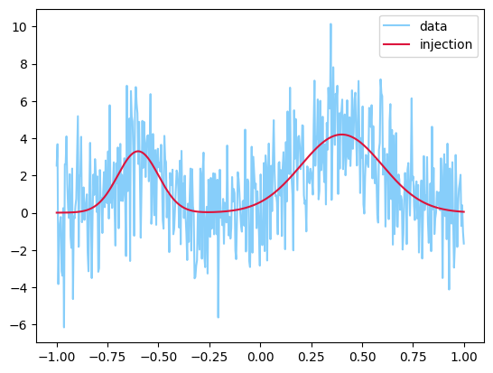
Now, we will build our GroupStretchMove that is based on the mean value of each Gaussian pulse.

from eryn.moves import GroupStretchMove

class MeanGaussianGroupMove(GroupStretchMove):
    def __init__(self, **kwargs):
        # make sure kwargs get sent into group stretch parent class
        GroupStretchMove.__init__(self, **kwargs)

    def setup_friends(self, branches):

        # store cold-chain information
        friends = branches["gauss"].coords[0, branches["gauss"].inds[0]]
        means = friends[:, 1].copy()  # need the copy

        # take unique to avoid errors at the start of sampling
        self.means, uni_inds = np.unique(means, return_index=True)
        self.friends = friends[uni_inds]

        # sort
        inds_sort = np.argsort(self.means)
        self.friends[:] = self.friends[inds_sort]
        self.means[:] = self.means[inds_sort]

        # get all current means from all temperatures
        current_means = branches["gauss"].coords[branches["gauss"].inds, 1]

        # calculate their distances to each stored friend
        dist = np.abs(current_means[:, None] - self.means[None, :])

        # get closest friends
        inds_closest = np.argsort(dist, axis=1)[:, : self.nfriends]

        # store in branch supplimental
        branches["gauss"].branch_supplimental[branches["gauss"].inds] = {
            "inds_closest": inds_closest
        }

        # make sure to "turn off" leaves that are deactivated by setting their
        # index to -1.
        branches["gauss"].branch_supplimental[~branches["gauss"].inds] = {
            "inds_closest": -np.ones(
                (ntemps, nwalkers, nleaves_max, self.nfriends), dtype=int
            )[~branches["gauss"].inds]
        }

    def fix_friends(self, branches):
        # when RJMCMC activates a new leaf, when it gets to this proposal, its inds_closest
        # will need to be updated

        # activated & does not have an assigned index
        fix = branches["gauss"].inds & (
            np.all(
                branches["gauss"].branch_supplimental[:]["inds_closest"] == -1,
                axis=-1,
            )
        )

        if not np.any(fix):
            return

        # same process as above, only for fix
        current_means = branches["gauss"].coords[fix, 1]

        dist = np.abs(current_means[:, None] - self.means[None, :])
        inds_closest = np.argsort(dist, axis=1)[:, : self.nfriends]

        branches["gauss"].branch_supplimental[fix] = {
            "inds_closest": inds_closest
        }

        # verify everything worked
        fix_check = branches["gauss"].inds & (
            np.all(
                branches["gauss"].branch_supplimental[:]["inds_closest"] == -1,
                axis=-1,
            )
        )
        assert not np.any(fix_check)

    def find_friends(self, name, s, s_inds=None, branch_supps=None):

        # prepare buffer array
        friends = np.zeros_like(s)

        # determine the closest friends for s_inds == True
        inds_closest_here = branch_supps[name][s_inds]["inds_closest"]

        # take one at random
        random_inds = inds_closest_here[
            np.arange(inds_closest_here.shape[0]),
            np.random.randint(
                self.nfriends, size=(inds_closest_here.shape[0],)
            ),
        ]

        # store in buffer array
        friends[s_inds] = self.friends[random_inds]
        return friends

# set random seed
np.random.seed(42)

nwalkers = 20
ntemps = 8
ndim = 3
nleaves_max = 5
nleaves_min = 0

branch_names = ["gauss"]

# initialize
nfriends = nwalkers
moves = MeanGaussianGroupMove(nfriends=nfriends, n_iters_update=200)

coords = {"gauss": np.zeros((ntemps, nwalkers, nleaves_max, ndim))}

# this is the sigma for the multivariate Gaussian that sets starting points
# We need it to be very small to assume we are passed the search phase
# we will verify this is with likelihood calculations
sig1 = 0.0001

# describes priors for all leaves independently
priors = {
    "gauss": ProbDistContainer(
        {
            0: uniform_dist(0.0, 10.0),  # amplitude
            1: uniform_dist(t.min(), t.max()),  # mean
            2: uniform_dist(0.01, 0.21),  # sigma
        }
    ),
}

# setup initial walkers as one starting guess
coords["gauss"][:, :, 0] = priors["gauss"].rvs(size=(ntemps, nwalkers))

inds = {"gauss": np.zeros((ntemps, nwalkers, nleaves_max), dtype=bool)}
inds["gauss"][:, :, 0] = True

# setup starting state
from eryn.state import BranchSupplemental

### KEY PART OF SETUP
# build branch supplimental to properly track information
# see below description of Branch Supplemental objects.
branch_supps = {
    "gauss": BranchSupplemental(
        {"inds_closest": np.zeros((ntemps, nwalkers, nleaves_max, nfriends), dtype=int)},
        base_shape=(ntemps, nwalkers, nleaves_max),
    )
}
state = State(
    coords,
    inds=inds,
    branch_supplimental=branch_supps,
)

ensemble = EnsembleSampler(
    nwalkers,
    ndim,
    log_like_fn_gauss_pulse,
    priors,
    args=[t, y, sigma],
    tempering_kwargs=dict(ntemps=ntemps),
    nbranches=len(branch_names),
    branch_names=branch_names,
    nleaves_max=nleaves_max,
    nleaves_min=nleaves_min,
    moves=moves,
    rj_moves=True,  # basic generation of new leaves from the prior
)

log_prior = ensemble.compute_log_prior(coords, inds=inds)
log_like = ensemble.compute_log_like(coords, inds=inds, logp=log_prior)[0]

state.log_prior = log_prior
state.log_like = log_like

nsteps = 100
last_sample = ensemble.run_mcmc(
    state, nsteps, burn=100, progress=True, thin_by=10
)

100%|█████████████████████████████████████████| 100/100 [00:02<00:00, 36.66it/s]
100%|███████████████████████████████████████| 1000/1000 [00:30<00:00, 32.88it/s]

Plot result. You may need to run this much longer to get a reasonable looking plot.

fig = corner.corner(
    ensemble.get_chain()["gauss"][:, 0][ensemble.get_inds()["gauss"][:, 0]],
    color="C1",
    hist_kwargs=dict(density=True),
    smooth=0.8,
)

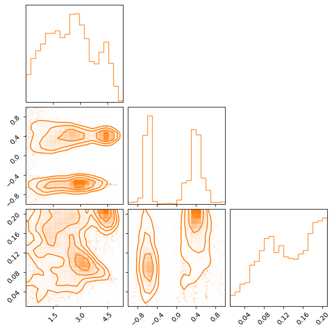
Utilities

Eryn provides many different utilities for sampling. We will show a bit of their usages here, but refer to the Utility documentation for more direct information.

Branch Supplemental

While the BranchSupplemental object is considered a utility, it is documented and stored within the section on the State objects (see here).

Sometimes, in sampling, we want to pass information through the sampler that is particular to each walker or leaf in our ensemble. Storing a different covariance matrix for each walker would be an example of this.

A BranchSupplemental object is designed to do this. In our example above on the GroupStretchMove, we used BranchSupplemental objects to hold and pass friend information through the sampler.

A major benefit of the branch supplimental is its indexing capabilities. As sampling proceeds, temperature swaps and accept/reject actions will change the current state coordinates and locations of each walker/leaf. The branch supplimental allows the sampling to track and move all of this extra information properly. For example, during a temperature swap, walker 0 in temperature 0 is swapped with walker 1 in temperature 1. This requires all information associated with (t,w)=(0, 0) to swap with walker information in (1,1). Eryn already does this directly for coordinates, inds, log like, log prior, etc. The branch supplimental ensures this swapping occurs properly for any other information you want to add that needs to track with each walker/leaf in the sampler.

from eryn.state import BranchSupplemental

BranchSupplemental objects are initialized with a dictionary with keys as names of the information and values as the array objects. These arrays can be dtype=object as well. This is discussed below. The base_shape gives the sampler shape of interest. Usually this is (ntemps, nwalkers, nleaves_max) or (ntemps, nwalkers). The indexing of the BranchSupplemental object will occur along this base_shape. It will return any dimensions beyond this base shape.

ntemps = 10
nwalkers = 30
nleaves_max = 12
n_info = 5

important_value = np.random.randint(1000, size=(ntemps, nwalkers, nleaves_max, n_info))
branch_supp = BranchSupplemental(
    {"important_value": important_value},
    base_shape=(ntemps, nwalkers, nleaves_max),
    copy=True
)

You can index and set the supplimental values in a simple way.

# index the object. It will return a dictionary.
print("BEFORE:", branch_supp[0, 1, 2], branch_supp[0, 1, 3])

# set the object with a dictionary
branch_supp[0, 1, 2] = {"important_value": np.array([1, 2, 3, 4, 5])}
print("AFTER:", branch_supp[0, 1, 2], branch_supp[0, 1, 3])

# set the object with another value (which is a dictionary)
branch_supp[0, 1, 2] = branch_supp[0, 1, 3]
print("AFTER2:", branch_supp[0, 1, 2], branch_supp[0, 1, 3])

BEFORE: {'important_value': array([ 52, 403, 967, 444, 130])} {'important_value': array([513, 587, 735, 702, 764])}
AFTER: {'important_value': array([1, 2, 3, 4, 5])} {'important_value': array([513, 587, 735, 702, 764])}
AFTER2: {'important_value': array([513, 587, 735, 702, 764])} {'important_value': array([513, 587, 735, 702, 764])}

BranchSupplemental objects are quietly powerful. You do not need to store numpy arrays as the supplimental. It can really be any object. Even, e.g., specialized class objects. In this case, you can store each class instance in a numpy array with dtype=object with base_shape=(ntemps, nwalkers, nleaves_max). Then, when indexing or adjusting, the branch supplimental will index as usual at the base_shape level.

class CarryAnything:
    def __init__(self, indicator, multiplier):
        self.indicator = indicator
        self.multiplier = multiplier

    def get_value(self):
        return self.indicator * self.multiplier

carry_any = []
for t in range(ntemps):
    for w in range(nwalkers):
        for l in range(nleaves_max):
            carry_any.append(CarryAnything(t * w, l))

carry_any = np.asarray(carry_any).reshape(ntemps, nwalkers, nleaves_max)
print(carry_any.shape)
print(carry_any[0, 0, :2])

(10, 30, 12)
[<__main__.CarryAnything object at 0x137cf54f0>
 <__main__.CarryAnything object at 0x1368f4b30>]

The branch supplimental is now built simply with two key-value pairs in the input dictionary. Even though they have different overall shapes, the two inputs have the same base_shape and can be indexed together properly.

branch_supp_inputs = {
    "important_value": important_value,
    "carry_any": carry_any
}

branch_supp = BranchSupplemental(
    branch_supp_inputs,
    base_shape=(ntemps, nwalkers, nleaves_max),
    copy=True
)

print(branch_supp[0, 1, 2])
print(branch_supp[5, 1, 2]["carry_any"].get_value())

{'important_value': array([ 52, 403, 967, 444, 130]), 'carry_any': <__main__.CarryAnything object at 0x135204dd0>}
10

For direct access to the holder arrays, you can access the holder attribute.

branch_supp.holder.keys()

dict_keys(['important_value', 'carry_any'])

Transform Container

Transform containers are primary used in likelihood functions to transform the arrays incoming from the sampler to the proper setup for likelihood computation. It can transform parameters based on transform functions and fill values into a final array for any value that is fixed during sampling.

It can be passed to the likeihood function as an arg or kwarg.

# can be done with lambda or regular function
# must have same number of inputs and outputs at same index in outer arrays
def transform1(x, y):
    return x * y, y / x

# this will do transform lambda x, y: (x**2, y**2) before transform1
parameter_transforms = {0: lambda x: np.log(x), (1, 2): lambda x, y: (x**2, y**2), (0, 2): transform1}

fill_dict = {
    "ndim_full": 6,  # full dimensionality after values are added
    "fill_inds": np.array([2, 3, 5]),  # indexes for fill values in final array
    "fill_values": np.array([0.0, 1.0, -1.0]),  # associated values for filling
}

tc = TransformContainer(parameter_transforms=parameter_transforms, fill_dict=fill_dict)

x = np.random.uniform(0.1, 4.0, size=(40, 3))

# can copy and transpose values if needed
out = tc.transform_base_parameters(x, copy=True, return_transpose=False)
print(out)

[[ 2.26227781e+00  7.71172976e+00  1.27548736e+00]
 [ 2.56370157e+00  1.34990453e-01  2.05917997e+00]
 [-1.48759469e+00  9.74032231e+00 -5.81326542e+01]
 [ 6.50447002e-02  1.63975125e+00  1.46380376e+00]
 [ 9.53877519e+00  7.79897194e-02  2.09789713e+01]
 [ 4.06410029e+00  1.26998074e+01  3.49285015e+00]
 [ 1.54376007e+01  1.38051140e+01  8.84060841e+00]
 [ 1.38300414e+01  2.53601577e+00  1.75672789e+01]
 [ 1.73703931e+00  9.27046560e+00  2.46312421e+01]
 [ 4.78771247e-01  3.75305760e+00  1.06581635e+00]
 [ 1.88147701e-02  2.34955242e-02  3.94187130e-02]
 [ 1.71883744e+01  2.54740727e-02  8.97001618e+00]
 [ 5.98474438e+00  3.00342614e+00  5.88277683e+00]
 [ 6.32764883e+00  2.34138626e-01  4.35158910e+00]
 [ 3.83219365e+00  1.24534275e+01  1.02614546e+01]
 [ 1.97048601e-01  1.66615073e+00  4.51228417e+00]
 [ 9.76220395e+00  1.16789539e+01  1.26683150e+01]
 [ 4.82678472e+00  3.07381945e+00  8.61128946e+00]
 [ 1.69598253e+00  1.18751365e+01  2.01722672e+01]
 [ 1.07081046e+00  1.53621702e+01  1.11803061e+00]
 [ 3.16326742e+00  4.02708000e+00  4.10980080e+00]
 [ 4.45485130e+00  3.87056124e+00  3.05496019e+00]
 [-5.96313442e-01  1.35690268e+01 -1.54661617e+00]
 [ 3.11288581e+00  6.68544747e-01  2.69885225e+00]
 [ 4.11935523e+00  6.96904238e+00  7.91590796e+00]
 [ 3.06494985e+00  2.75972186e-01  3.14017465e+01]
 [ 1.87475913e+01  3.91251640e-01  1.16695627e+01]
 [ 2.66873057e-01  7.02594142e+00  1.45960933e-01]
 [ 5.33294936e+00  6.11129950e+00  3.22032393e+00]
 [-1.02392877e+00  3.86543400e-01 -4.37596988e+00]
 [ 3.18067491e+00  8.25836145e-01  1.33798856e+01]
 [ 5.62668854e+00  9.78027707e+00  3.52857318e+00]
 [-5.99820781e-02  4.79023757e+00 -3.70779337e-01]
 [ 3.62128048e+00  8.37144246e+00  1.07501880e+01]
 [ 3.95266270e-01  7.04161418e-01  2.02500595e+00]
 [ 1.34621385e+01  7.98391055e-01  9.13549746e+00]
 [-1.34151067e+01  8.40039254e+00 -3.57508963e+00]
 [ 8.54177631e+00  9.17191891e+00  6.84911323e+00]
 [-2.07751004e+01  6.12957529e+00 -6.70874225e+00]
 [ 8.48004061e+00  1.06033804e+01  5.51752276e+00]]

If you have mutliple branches in your sampler, you can add more than one Transform Container.

def lnprob(x1, group1, x2, group2, transform_containers):
    x = [x1, x2]
    for i, (x_i, transform) in enumerate(zip([x1, x2], transform_containers)):
        temp = transform.transform_base_parameters(x_i, copy=True, return_transpose=False)
        x[i] = transform.fill_values(temp)

    print(x)

    ## do more in the likelihood here with transformed information

# setup transforms for x1
parameter_transforms1 = {0: lambda x: np.log(x)}

# setup transforms for x2
parameter_transforms2 = {(1, 2): lambda x, y: (x**2, y**2)}

# fill dict for x1
fill_dict1 = {
    "ndim_full": 6,  # full dimensionality after values are added
    "fill_inds": np.array([2, 3, 5]),  # indexes for fill values in final array
    "fill_values": np.array([0.0, 1.0, -1.0]),  # associated values for filling
}

# fill dict for x2
fill_dict2 = {
    "ndim_full": 5,  # full dimensionality after values are added
    "fill_inds": np.array([1]),  # indexes for fill values in final array
    "fill_values": np.array([-1.0]),  # associated values for filling
}

tcs = [
    TransformContainer(parameter_transforms=parameter_transforms1, fill_dict=fill_dict1),
    TransformContainer(parameter_transforms=parameter_transforms2, fill_dict=fill_dict2),
]

num = 40
x1 = np.random.uniform(0.1, 4.0, size=(num, 3))
x2 = np.random.uniform(0.1, 4.0, size=(num, 4))

group1 = np.arange(num)
group2 = np.arange(num)

# it can be added via args or kwargs in the ensemble sampler
lnprob(x1, group1, x2, group2, tcs)

[array([[ 1.36408262,  0.15052344,  0.        ,  1.        ,  3.48800761,
        -1.        ],
       [ 1.29897891,  3.01041913,  0.        ,  1.        ,  2.97851441,
        -1.        ],
       [ 1.3653482 ,  1.21394415,  0.        ,  1.        ,  3.25311149,
        -1.        ],
       [ 1.16750397,  2.64909661,  0.        ,  1.        ,  1.45690912,
        -1.        ],
       [ 1.1861526 ,  0.93322534,  0.        ,  1.        ,  3.58088928,
        -1.        ],
       [ 0.08555872,  0.13786158,  0.        ,  1.        ,  3.43834971,
        -1.        ],
       [-0.02352741,  1.71808764,  0.        ,  1.        ,  3.63735008,
        -1.        ],
       [ 1.07232766,  1.39277427,  0.        ,  1.        ,  0.63799694,
        -1.        ],
       [ 1.21732595,  3.14024127,  0.        ,  1.        ,  0.69714093,
        -1.        ],
       [ 0.26845662,  2.84958172,  0.        ,  1.        ,  1.44775212,
        -1.        ],
       [ 0.55606073,  3.12060581,  0.        ,  1.        ,  3.68667253,
        -1.        ],
       [ 0.97680555,  3.65644994,  0.        ,  1.        ,  3.39990504,
        -1.        ],
       [ 0.63347517,  2.07772332,  0.        ,  1.        ,  3.32185317,
        -1.        ],
       [ 0.54807996,  1.63004179,  0.        ,  1.        ,  3.63537474,
        -1.        ],
       [ 0.78315515,  1.74865946,  0.        ,  1.        ,  2.72034487,
        -1.        ],
       [ 0.62543905,  3.89346839,  0.        ,  1.        ,  3.81664149,
        -1.        ],
       [ 0.25188632,  2.9573227 ,  0.        ,  1.        ,  1.29585671,
        -1.        ],
       [-0.07794654,  0.24376449,  0.        ,  1.        ,  2.28643517,
        -1.        ],
       [ 1.05373448,  1.80619337,  0.        ,  1.        ,  0.49407366,
        -1.        ],
       [ 0.61174823,  0.25112653,  0.        ,  1.        ,  1.49639733,
        -1.        ],
       [ 1.14970147,  2.03962511,  0.        ,  1.        ,  1.01071637,
        -1.        ],
       [ 1.17866892,  3.44375584,  0.        ,  1.        ,  2.89257887,
        -1.        ],
       [ 1.25003678,  3.97263296,  0.        ,  1.        ,  2.28063182,
        -1.        ],
       [ 1.28028481,  2.67240503,  0.        ,  1.        ,  1.88979263,
        -1.        ],
       [ 0.93052516,  0.98698515,  0.        ,  1.        ,  1.49915708,
        -1.        ],
       [ 1.28665103,  0.94348679,  0.        ,  1.        ,  2.8971265 ,
        -1.        ],
       [ 0.80048835,  0.22247766,  0.        ,  1.        ,  2.58255823,
        -1.        ],
       [ 0.68911496,  3.48062074,  0.        ,  1.        ,  1.04180256,
        -1.        ],
       [ 1.04477123,  2.76761527,  0.        ,  1.        ,  1.8895895 ,
        -1.        ],
       [ 1.11761682,  3.51274366,  0.        ,  1.        ,  1.03211138,
        -1.        ],
       [ 1.35853643,  0.74031876,  0.        ,  1.        ,  3.07061094,
        -1.        ],
       [ 1.25215733,  3.22604585,  0.        ,  1.        ,  2.32227826,
        -1.        ],
       [-1.65465746,  2.10116328,  0.        ,  1.        ,  3.74740296,
        -1.        ],
       [ 1.13880739,  2.16460269,  0.        ,  1.        ,  1.08915955,
        -1.        ],
       [ 1.28951076,  1.33559827,  0.        ,  1.        ,  1.35421215,
        -1.        ],
       [-0.42504646,  3.91291818,  0.        ,  1.        ,  1.41934187,
        -1.        ],
       [-0.98377096,  0.81228842,  0.        ,  1.        ,  2.83893009,
        -1.        ],
       [ 0.94390451,  0.31438458,  0.        ,  1.        ,  3.08240101,
        -1.        ],
       [ 1.07355977,  3.06460086,  0.        ,  1.        ,  1.02755997,
        -1.        ],
       [ 0.73020403,  2.47933908,  0.        ,  1.        ,  0.73662634,
        -1.        ]]), array([[ 1.12687226, -1.        ,  4.00248679,  2.53636448,  3.8903226 ],
       [ 3.85913129, -1.        ,  0.34563185,  1.14920481,  3.36494113],
       [ 0.96183002, -1.        ,  8.16346346,  7.04960439,  3.69095477],
       [ 1.70945362, -1.        ,  0.35545822,  0.03237407,  1.46548275],
       [ 2.26824275, -1.        ,  8.97436765,  4.87113036,  2.22131114],
       [ 1.35178665, -1.        ,  7.83610769,  5.20127569,  0.10671333],
       [ 2.87588294, -1.        , 14.34902369,  0.24361026,  3.46439266],
       [ 0.93154318, -1.        ,  4.12893585,  4.46943857,  0.60840224],
       [ 1.24729566, -1.        ,  0.1734498 ,  4.79654616,  3.91285921],
       [ 2.51556969, -1.        , 14.3047392 ,  0.6397266 ,  2.44207147],
       [ 3.20962925, -1.        ,  2.60030366,  0.19040972,  3.1133263 ],
       [ 2.08560979, -1.        ,  0.62009154,  0.05022364,  2.40225947],
       [ 0.33199571, -1.        ,  0.03074056,  5.71869472,  2.15882122],
       [ 1.47946504, -1.        ,  1.87289675,  0.90151358,  0.24074501],
       [ 2.9770715 , -1.        ,  4.79907015, 12.43276481,  1.65995714],
       [ 3.74138046, -1.        ,  4.22514186,  2.34456864,  2.56201691],
       [ 1.78500232, -1.        ,  1.31720371,  6.57318376,  2.34359725],
       [ 2.00965002, -1.        ,  0.14123776, 11.47295327,  2.03166857],
       [ 3.33775044, -1.        ,  0.16989541,  4.13695376,  2.89669478],
       [ 1.09487498, -1.        , 13.55598354,  2.22904415,  1.51427016],
       [ 0.70048696, -1.        ,  1.23266067, 11.64083866,  2.08934512],
       [ 1.35181021, -1.        ,  9.42599021,  7.28069835,  1.97750598],
       [ 0.3435387 , -1.        , 15.7217224 ,  0.68781272,  1.99812126],
       [ 2.98962262, -1.        ,  4.42467445,  9.79329395,  2.63975936],
       [ 2.49725691, -1.        , 11.14015574, 11.38180071,  0.4340989 ],
       [ 0.9915848 , -1.        ,  9.50677174, 15.1801135 ,  2.0664768 ],
       [ 3.05431651, -1.        ,  3.60922715, 12.52595309,  2.06785213],
       [ 1.0526226 , -1.        ,  9.74426111,  2.43847953,  0.37556454],
       [ 0.55103816, -1.        , 11.7703627 , 11.19127215,  1.61686159],
       [ 3.83934958, -1.        ,  3.69902273, 11.75327062,  3.54293484],
       [ 2.31728036, -1.        ,  0.27001597,  2.77863309,  2.83587134],
       [ 0.23100948, -1.        ,  2.44550709,  3.61791316,  2.31107967],
       [ 3.38838798, -1.        ,  1.60084254,  0.62853765,  3.54487269],
       [ 2.74178253, -1.        ,  1.76503062,  0.75122448,  3.05916718],
       [ 2.90819838, -1.        , 12.59782578,  9.7869203 ,  3.82881016],
       [ 3.52381286, -1.        ,  1.63105348, 10.28011431,  2.25903713],
       [ 3.89240716, -1.        ,  2.75460847,  2.91276999,  0.68357577],
       [ 3.49780335, -1.        ,  1.47979089, 15.00484949,  2.3351851 ],
       [ 2.18227792, -1.        ,  7.10108032,  0.59811628,  0.10842801],
       [ 1.46135392, -1.        ,  6.58120056,  0.42250042,  2.99398862]])]

Multivariate Prior Distributions

Eryn also allows for multivariate prior distributions. To pass these, rather than a single index as the dictionary key like before (e.g.1: dist()), it is not a tuple of inds: (0, 1): dist().

from scipy.stats import multivariate_normal
cov = np.array([[0.8, -0.2], [-0.2, 0.4]])

priors_in = {
    (0, 1): multivariate_normal(cov=cov)
}
priors = ProbDistContainer(priors_in)
prior_vals = priors.rvs(size=12)
print(prior_vals.shape)

(12, 2)

Periodic Container

The periodic container accounts for periodic parameters by accounting for periodic boundary conditions in terms of distance and parameter wrapping. The input to periodic containers are dictionaries with the parameter index as the key and the period associated with it as the item. Any parameters that are not periodic do not need to be included.

For example, with a sine model that includes an amplitude (index 0), frequency (index 1), and phase offset (index 2), the phase offset will be periodic.

from eryn.utils import PeriodicContainer


periodic = PeriodicContainer({"sine": {2: 2 * np.pi}})
ntemps, nwalkers, nleaves_max, ndim = (10, 100, 2, 3)

params_before_1 = {"sine": np.random.uniform(0, 7.0, size=(ntemps * nwalkers, nleaves_max, ndim))}
params_before_2 = {"sine": np.random.uniform(0, 7.0, size=(ntemps * nwalkers, nleaves_max, ndim))}

distance = periodic.distance(params_before_1, params_before_2)

# the max distance should be near half the period
print(distance["sine"][:, :, -1].max())

params_after_1 = periodic.wrap(params_before_1)

# max after wrapping should be near the period
print(params_after_1["sine"][:, :, -1].max())

3.1396228175679486
6.281999449819018

Stopping & Update Functions

Stopping and Update functions are built, declared, and adjusted in the same way. They both have required Parent base classes. The key similarity between them is the __call__ function has the same signature: (iteration, last_sample, sampler), which gives the class access to the all parts of the sampler object.

Update functions allow the user to adjust anything within the sampler at periodic intervals set by the update_iterations kwarg to EnsembleSampler. This can also be used to access very types of information. It allows for a ton of customization from the user from within the sampler object. See the update documentation for more information.

Stopping functions are effectively convergence functions, allowing the sampler to stop running when it reaches a user-defined criterion. For more information, see the stopping documentation.

Here, we will just look at a quick example of using the implemented stopping function for Likelihood convergence.

from eryn.utils import SearchConvergeStopping

# Gaussian likelihood
def log_like_fn(x, mu, invcov):
    diff = x - mu
    return -0.5 * (diff * np.dot(invcov, diff.T).T).sum()

ndim = 5
nwalkers = 100

# mean
means = np.zeros(ndim)  # np.random.rand(ndim)

# define covariance matrix
cov = np.diag(np.ones(ndim))
invcov = np.linalg.inv(cov)

# set prior limits
lims = 50.0
priors_in = {i: uniform_dist(-lims + means[i], lims + means[i]) for i in range(ndim)}
priors = ProbDistContainer(priors_in)

stop = SearchConvergeStopping(n_iters=5, diff=0.01, verbose=True)

ensemble = EnsembleSampler(
    nwalkers,
    ndim,
    log_like_fn,
    priors,
    args=[means, invcov],
    stopping_fn=stop,
    stopping_iterations=5
)

# starting positions
# randomize throughout prior
coords = priors.rvs(size=(nwalkers,))

# check log_like
log_like = np.asarray([
    log_like_fn(coords[i], means, invcov)
for i in range(nwalkers)])
print(log_like)

# check log_prior
log_prior = np.asarray([
    priors.logpdf(coords[i])
for i in range(nwalkers)])
print(log_prior)


nsteps = 500
# burn for 1000 steps
burn = 100
# thin by 5
thin_by = 5
out = ensemble.run_mcmc(coords, nsteps, burn=burn, progress=True, thin_by=thin_by)

[-1640.49679761 -2135.49803152 -1902.77160243 -2518.77462291
 -2051.94825594 -2318.71684266 -1845.07485743 -1575.80578615
  -913.80921413 -1108.9449725  -1780.20151453  -979.04011531
 -1885.25829617  -772.78021174 -4961.74355071  -651.92498531
 -4058.42587146 -2222.75261641 -2587.35271764 -2888.26717103
 -2385.10797455 -1067.19887104 -4170.31900754 -3081.79590684
 -1711.62977293 -1921.02255461 -1647.87020108 -1350.79724116
 -1635.07917685 -2978.59460227 -3025.81761755 -2465.65385449
 -1584.44439791  -705.24033014 -2265.53587807 -1800.29764511
 -2211.43468005 -2932.15312204 -2036.16814252 -3251.00408331
 -2218.88843675 -1989.9393407  -1387.18420155 -1249.69733655
 -3231.91216326 -2128.41154584 -1266.54584638 -1738.55937653
 -1474.89128224 -1208.04481689 -2817.42974363 -2230.42847214
 -1881.77767607 -3321.4775246  -1310.57188017 -1404.39592594
 -2688.28462417 -1035.47864803 -1691.88082256 -2441.60925324
 -2263.23620765 -1706.78581038 -1752.00845384 -2282.29407206
 -1137.81695955 -3564.67451667 -2363.60233296 -2000.43831628
 -2028.68778873 -1129.81047553 -2766.82574299  -417.17183832
 -1917.548434   -1166.39969534 -2138.33358483 -1225.25105585
 -1110.89568937  -940.52124789 -1155.42212252 -1835.39263386
 -3442.64290351 -2734.30955334 -1944.82023546 -2678.47097937
 -1191.16174763 -2395.23521606 -2151.11201375 -2164.7197384
 -3467.95403029 -1675.31598053 -3367.0266415  -1295.71312178
 -2383.21420848 -3324.94357378 -2177.44460386 -1041.76021323
  -886.82478613 -1698.56702022 -2270.08719732 -2844.77627149]
[-23.02585093 -23.02585093 -23.02585093 -23.02585093 -23.02585093
 -23.02585093 -23.02585093 -23.02585093 -23.02585093 -23.02585093
 -23.02585093 -23.02585093 -23.02585093 -23.02585093 -23.02585093
 -23.02585093 -23.02585093 -23.02585093 -23.02585093 -23.02585093
 -23.02585093 -23.02585093 -23.02585093 -23.02585093 -23.02585093
 -23.02585093 -23.02585093 -23.02585093 -23.02585093 -23.02585093
 -23.02585093 -23.02585093 -23.02585093 -23.02585093 -23.02585093
 -23.02585093 -23.02585093 -23.02585093 -23.02585093 -23.02585093
 -23.02585093 -23.02585093 -23.02585093 -23.02585093 -23.02585093
 -23.02585093 -23.02585093 -23.02585093 -23.02585093 -23.02585093
 -23.02585093 -23.02585093 -23.02585093 -23.02585093 -23.02585093
 -23.02585093 -23.02585093 -23.02585093 -23.02585093 -23.02585093
 -23.02585093 -23.02585093 -23.02585093 -23.02585093 -23.02585093
 -23.02585093 -23.02585093 -23.02585093 -23.02585093 -23.02585093
 -23.02585093 -23.02585093 -23.02585093 -23.02585093 -23.02585093
 -23.02585093 -23.02585093 -23.02585093 -23.02585093 -23.02585093
 -23.02585093 -23.02585093 -23.02585093 -23.02585093 -23.02585093
 -23.02585093 -23.02585093 -23.02585093 -23.02585093 -23.02585093
 -23.02585093 -23.02585093 -23.02585093 -23.02585093 -23.02585093
 -23.02585093 -23.02585093 -23.02585093 -23.02585093 -23.02585093]

100%|████████████████████████████████████████| 100/100 [00:00<00:00, 291.24it/s]
  3%|█                                       | 63/2500 [00:00<00:07, 314.42it/s]

ITERS CONSECUTIVE: 0 Previous best LL: -0.09111836076165353 Current best LL: -0.09111836076165353


ITERS CONSECUTIVE: 1 Previous best LL: -0.09111836076165353 Current best LL: -0.09111836076165353


ITERS CONSECUTIVE: 2 Previous best LL: -0.09111836076165353 Current best LL: -0.09111836076165353

  6%|██▍                                    | 157/2500 [00:00<00:07, 296.77it/s]

ITERS CONSECUTIVE: 0 Previous best LL: -0.0742244529294836 Current best LL: -0.0742244529294836


ITERS CONSECUTIVE: 1 Previous best LL: -0.0742244529294836 Current best LL: -0.0742244529294836


ITERS CONSECUTIVE: 2 Previous best LL: -0.0742244529294836 Current best LL: -0.0742244529294836

  9%|███▍                                   | 217/2500 [00:00<00:07, 286.14it/s]

ITERS CONSECUTIVE: 3 Previous best LL: -0.0742244529294836 Current best LL: -0.07399422624832219


ITERS CONSECUTIVE: 0 Previous best LL: -0.04450561782490035 Current best LL: -0.04450561782490035


ITERS CONSECUTIVE: 1 Previous best LL: -0.04450561782490035 Current best LL: -0.04450561782490035

 12%|████▊                                  | 305/2500 [00:01<00:07, 286.26it/s]

ITERS CONSECUTIVE: 2 Previous best LL: -0.04450561782490035 Current best LL: -0.04450561782490035


ITERS CONSECUTIVE: 3 Previous best LL: -0.04450561782490035 Current best LL: -0.04450561782490035


ITERS CONSECUTIVE: 4 Previous best LL: -0.04450561782490035 Current best LL: -0.04450561782490035

 13%|█████                                  | 325/2500 [00:01<00:07, 287.83it/s]

ITERS CONSECUTIVE: 5 Previous best LL: -0.04450561782490035 Current best LL: -0.04450561782490035