Introduction
LISA Analysis Tools is a group of code packages that brings together many different aspects of LISA data analysis. In this tutorial, we will describe the functionality of the main high-level package: lisatools. This includes defining sensitivity, orbit, and other information. Also, this includes computing many basic waveform-level diagnostics.
The documentation for lisatools can be found here.
If you use this code, please cite the zenodo.
[1]:
import matplotlib.pyplot as plt
import numpy as np

from eryn.utils import TransformContainer

from lisatools.sensitivity import *
from lisatools.utils.constants import *
from lisatools.diagnostic import *
from lisatools.detector import EqualArmlengthOrbits, ESAOrbits
from lisatools.detector import LISAModel
from lisatools.detector import get_available_default_lisa_models
from lisatools.detector import scirdv1
LISA Sensitivity
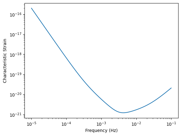
We will begin with generating the LISA sensitivity. You can do this with the lisatools.sensitivity.get_sensitivity function. Some helpful keyword arguments:
sens_fn: Type of sensitivity response function. Base sensitivity or TDI sensitivity. Base sensitivity:LISASens. TDI sensitivities are shown below.return_type: PSD, ASD, or characteristic strain.
[2]:
f = np.logspace(-5, -1, 10000)
Sn = get_sensitivity(f, sens_fn=LISASens, return_type="char_strain")
plt.loglog(f, Sn)
plt.xlabel("Frequency (Hz)")
plt.ylabel("Characteristic Strain")
[2]:
Text(0, 0.5, 'Characteristic Strain')
Stock sensitivity options can be found with lisatools.sensitivity.get_stock_sensitivity_options.
[3]:
from lisatools.sensitivity import get_stock_sensitivity_options
[4]:
get_stock_sensitivity_options()
[4]:
['X1TDISens',
 'Y1TDISens',
 'Z1TDISens',
 'XY1TDISens',
 'YZ1TDISens',
 'ZX1TDISens',
 'A1TDISens',
 'E1TDISens',
 'T1TDISens',
 'X2TDISens',
 'Y2TDISens',
 'Z2TDISens',
 'XY2TDISens',
 'YZ2TDISens',
 'ZX2TDISens',
 'LISASens',
 'CornishLISASens',
 'FlatPSDFunction']
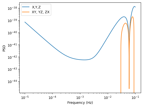
PSD for TDI channels X,Y,Z
Plot the TDI X,Y,Z channels (X1TDISens, Y1TDISens, Z1TDISens) and cross-sensitivity (XY1TDISens, YZ1TDISens, ZX1TDISens). The “1” here represents TDI generation 1. TDI 2 is available, but not the cross-terms yet. They need to be added.
[5]:
f = np.logspace(-5, -1, 10000)
Sn = get_sensitivity(f, sens_fn=X1TDISens, return_type="PSD")
plt.loglog(f, Sn, label="X,Y,Z")
Cn = get_sensitivity(f, sens_fn=XY1TDISens, return_type="PSD")
plt.loglog(f, Cn, label="XY, YZ, ZX")
plt.legend()
plt.xlabel("Frequency (Hz)")
plt.ylabel("PSD")
[5]:
Text(0, 0.5, 'PSD')
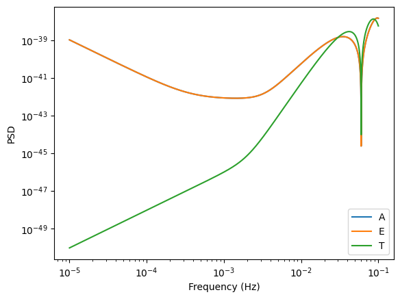
PSD for TDI channels A,E,T
Similary now for TDI A,E,T channels.
[6]:
f = np.logspace(-5, -1, 10000)
SnA = get_sensitivity(f, sens_fn=A1TDISens, return_type="PSD")
SnE = get_sensitivity(f, sens_fn=E1TDISens, return_type="PSD")
SnT = get_sensitivity(f, sens_fn=T1TDISens, return_type="PSD")
plt.loglog(f, SnA, label="A")
plt.loglog(f, SnE, label="E")
plt.loglog(f, SnT, label="T")
plt.xlabel("Frequency (Hz)")
plt.legend()
plt.ylabel("PSD")
[6]:
Text(0, 0.5, 'PSD')
Sensitivity Matrices
Sensitivity Matrices create a holder for sensitivity information across different channels. It allows for a common backend to be fed to diagnostic functions regardless if you are using AET in a length 3 array, XYZ in 3x3 matrix, or a set of basic LISASens objects. Sensitivity matrices can plot your sensitivity and update information on the fly (like if the frequency changes).
Here is a custom version of a 3x3 sensitivity matrix.
[7]:
sens_mat = SensitivityMatrix(
    f,
    [
        [X1TDISens, XY1TDISens, ZX1TDISens],
        [XY1TDISens, Y1TDISens, YZ1TDISens],
        [ZX1TDISens, YZ1TDISens, Z1TDISens],
    ],
    stochastic_params=(1.0 * YRSID_SI,),
    model=lisa_models.scirdv1,
)
You can see the stock SensitivityMatrix options with lisatools.sensitivity.get_stock_sensitivity_matrix_options.
[8]:
from lisatools.sensitivity import get_stock_sensitivity_matrix_options
[9]:
get_stock_sensitivity_matrix_options()
[9]:
['XYZ1SensitivityMatrix',
 'XYZ2SensitivityMatrix',
 'AET1SensitivityMatrix',
 'AE1SensitivityMatrix']
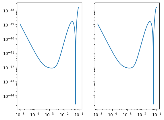
[10]:
sens_mat2 = AE1SensitivityMatrix(
    f,
    # stochastic_params=None, (1.0 * YRSID_SI,),
    model=lisa_models.scirdv1,
)

sens_mat2.loglog()
[10]:
(<Figure size 640x480 with 2 Axes>, array([<Axes: >, <Axes: >], dtype=object))
You can adjust the frequencies, model, or stochastic information (see below for Stochastic) with the methods that start with “update.” For the frequency:
[11]:
sens_mat2.update_frequency_arr(np.logspace(-4, -1, 1000))
[12]:
sens_mat2.frequency_arr
[12]:
array([0.0001    , 0.00010069, 0.00010139, 0.0001021 , 0.0001028 ,
       0.00010352, 0.00010424, 0.00010496, 0.00010569, 0.00010642,
       0.00010716, 0.0001079 , 0.00010865, 0.00010941, 0.00011016,
       0.00011093, 0.0001117 , 0.00011247, 0.00011325, 0.00011404,
       0.00011483, 0.00011563, 0.00011643, 0.00011724, 0.00011805,
       0.00011887, 0.0001197 , 0.00012053, 0.00012136, 0.0001222 ,
       0.00012305, 0.00012391, 0.00012477, 0.00012563, 0.0001265 ,
       0.00012738, 0.00012826, 0.00012915, 0.00013005, 0.00013095,
       0.00013186, 0.00013278, 0.0001337 , 0.00013463, 0.00013556,
       0.0001365 , 0.00013745, 0.0001384 , 0.00013936, 0.00014033,
       0.0001413 , 0.00014228, 0.00014327, 0.00014426, 0.00014527,
       0.00014627, 0.00014729, 0.00014831, 0.00014934, 0.00015038,
       0.00015142, 0.00015247, 0.00015353, 0.00015459, 0.00015567,
       0.00015675, 0.00015783, 0.00015893, 0.00016003, 0.00016114,
       0.00016226, 0.00016339, 0.00016452, 0.00016566, 0.00016681,
       0.00016797, 0.00016913, 0.00017031, 0.00017149, 0.00017268,
       0.00017388, 0.00017508, 0.0001763 , 0.00017752, 0.00017875,
       0.00017999, 0.00018124, 0.0001825 , 0.00018377, 0.00018504,
       0.00018632, 0.00018762, 0.00018892, 0.00019023, 0.00019155,
       0.00019288, 0.00019422, 0.00019557, 0.00019692, 0.00019829,
       0.00019966, 0.00020105, 0.00020244, 0.00020385, 0.00020526,
       0.00020669, 0.00020812, 0.00020957, 0.00021102, 0.00021248,
       0.00021396, 0.00021544, 0.00021694, 0.00021844, 0.00021996,
       0.00022149, 0.00022302, 0.00022457, 0.00022613, 0.0002277 ,
       0.00022928, 0.00023087, 0.00023247, 0.00023408, 0.00023571,
       0.00023734, 0.00023899, 0.00024065, 0.00024232, 0.000244  ,
       0.00024569, 0.0002474 , 0.00024911, 0.00025084, 0.00025258,
       0.00025433, 0.0002561 , 0.00025788, 0.00025967, 0.00026147,
       0.00026328, 0.00026511, 0.00026695, 0.0002688 , 0.00027067,
       0.00027254, 0.00027443, 0.00027634, 0.00027826, 0.00028019,
       0.00028213, 0.00028409, 0.00028606, 0.00028804, 0.00029004,
       0.00029206, 0.00029408, 0.00029612, 0.00029818, 0.00030025,
       0.00030233, 0.00030443, 0.00030654, 0.00030867, 0.00031081,
       0.00031296, 0.00031514, 0.00031732, 0.00031952, 0.00032174,
       0.00032397, 0.00032622, 0.00032849, 0.00033076, 0.00033306,
       0.00033537, 0.0003377 , 0.00034004, 0.0003424 , 0.00034478,
       0.00034717, 0.00034958, 0.000352  , 0.00035445, 0.0003569 ,
       0.00035938, 0.00036187, 0.00036439, 0.00036691, 0.00036946,
       0.00037202, 0.00037461, 0.0003772 , 0.00037982, 0.00038246,
       0.00038511, 0.00038778, 0.00039047, 0.00039318, 0.00039591,
       0.00039866, 0.00040142, 0.00040421, 0.00040701, 0.00040984,
       0.00041268, 0.00041555, 0.00041843, 0.00042133, 0.00042426,
       0.0004272 , 0.00043016, 0.00043315, 0.00043615, 0.00043918,
       0.00044223, 0.0004453 , 0.00044839, 0.0004515 , 0.00045463,
       0.00045778, 0.00046096, 0.00046416, 0.00046738, 0.00047062,
       0.00047389, 0.00047718, 0.00048049, 0.00048382, 0.00048718,
       0.00049056, 0.00049396, 0.00049739, 0.00050084, 0.00050432,
       0.00050782, 0.00051134, 0.00051489, 0.00051846, 0.00052206,
       0.00052568, 0.00052933, 0.000533  , 0.0005367 , 0.00054042,
       0.00054417, 0.00054795, 0.00055175, 0.00055558, 0.00055943,
       0.00056331, 0.00056722, 0.00057116, 0.00057512, 0.00057911,
       0.00058313, 0.00058718, 0.00059125, 0.00059535, 0.00059948,
       0.00060364, 0.00060783, 0.00061205, 0.0006163 , 0.00062057,
       0.00062488, 0.00062921, 0.00063358, 0.00063798, 0.0006424 ,
       0.00064686, 0.00065135, 0.00065587, 0.00066042, 0.000665  ,
       0.00066962, 0.00067426, 0.00067894, 0.00068365, 0.0006884 ,
       0.00069317, 0.00069798, 0.00070282, 0.0007077 , 0.00071261,
       0.00071756, 0.00072253, 0.00072755, 0.0007326 , 0.00073768,
       0.0007428 , 0.00074795, 0.00075314, 0.00075837, 0.00076363,
       0.00076893, 0.00077426, 0.00077964, 0.00078505, 0.00079049,
       0.00079598, 0.0008015 , 0.00080706, 0.00081266, 0.0008183 ,
       0.00082398, 0.0008297 , 0.00083545, 0.00084125, 0.00084709,
       0.00085296, 0.00085888, 0.00086484, 0.00087084, 0.00087689,
       0.00088297, 0.0008891 , 0.00089527, 0.00090148, 0.00090773,
       0.00091403, 0.00092037, 0.00092676, 0.00093319, 0.00093966,
       0.00094618, 0.00095275, 0.00095936, 0.00096602, 0.00097272,
       0.00097947, 0.00098627, 0.00099311, 0.001     , 0.00100694,
       0.00101393, 0.00102096, 0.00102804, 0.00103518, 0.00104236,
       0.00104959, 0.00105688, 0.00106421, 0.00107159, 0.00107903,
       0.00108652, 0.00109405, 0.00110165, 0.00110929, 0.00111699,
       0.00112474, 0.00113254, 0.0011404 , 0.00114831, 0.00115628,
       0.0011643 , 0.00117238, 0.00118052, 0.00118871, 0.00119696,
       0.00120526, 0.00121362, 0.00122204, 0.00123052, 0.00123906,
       0.00124766, 0.00125632, 0.00126503, 0.00127381, 0.00128265,
       0.00129155, 0.00130051, 0.00130954, 0.00131862, 0.00132777,
       0.00133698, 0.00134626, 0.0013556 , 0.00136501, 0.00137448,
       0.00138402, 0.00139362, 0.00140329, 0.00141303, 0.00142283,
       0.0014327 , 0.00144264, 0.00145265, 0.00146273, 0.00147288,
       0.0014831 , 0.00149339, 0.00150376, 0.00151419, 0.0015247 ,
       0.00153528, 0.00154593, 0.00155665, 0.00156746, 0.00157833,
       0.00158928, 0.00160031, 0.00161141, 0.0016226 , 0.00163385,
       0.00164519, 0.00165661, 0.0016681 , 0.00167967, 0.00169133,
       0.00170307, 0.00171488, 0.00172678, 0.00173876, 0.00175083,
       0.00176298, 0.00177521, 0.00178753, 0.00179993, 0.00181242,
       0.00182499, 0.00183766, 0.00185041, 0.00186325, 0.00187617,
       0.00188919, 0.0019023 , 0.0019155 , 0.00192879, 0.00194217,
       0.00195565, 0.00196922, 0.00198288, 0.00199664, 0.0020105 ,
       0.00202445, 0.00203849, 0.00205264, 0.00206688, 0.00208122,
       0.00209566, 0.0021102 , 0.00212485, 0.00213959, 0.00215443,
       0.00216938, 0.00218444, 0.00219959, 0.00221486, 0.00223022,
       0.0022457 , 0.00226128, 0.00227697, 0.00229277, 0.00230868,
       0.0023247 , 0.00234083, 0.00235707, 0.00237342, 0.00238989,
       0.00240648, 0.00242317, 0.00243999, 0.00245692, 0.00247396,
       0.00249113, 0.00250842, 0.00252582, 0.00254335, 0.00256099,
       0.00257876, 0.00259666, 0.00261467, 0.00263282, 0.00265108,
       0.00266948, 0.002688  , 0.00270665, 0.00272543, 0.00274434,
       0.00276339, 0.00278256, 0.00280187, 0.00282131, 0.00284088,
       0.0028606 , 0.00288044, 0.00290043, 0.00292056, 0.00294082,
       0.00296123, 0.00298177, 0.00300246, 0.00302329, 0.00304427,
       0.0030654 , 0.00308666, 0.00310808, 0.00312965, 0.00315136,
       0.00317323, 0.00319525, 0.00321742, 0.00323974, 0.00326222,
       0.00328486, 0.00330765, 0.0033306 , 0.00335371, 0.00337698,
       0.00340041, 0.00342401, 0.00344776, 0.00347169, 0.00349578,
       0.00352003, 0.00354446, 0.00356905, 0.00359381, 0.00361875,
       0.00364386, 0.00366914, 0.0036946 , 0.00372024, 0.00374605,
       0.00377204, 0.00379822, 0.00382457, 0.00385111, 0.00387783,
       0.00390474, 0.00393183, 0.00395911, 0.00398658, 0.00401424,
       0.0040421 , 0.00407014, 0.00409838, 0.00412682, 0.00415546,
       0.00418429, 0.00421332, 0.00424256, 0.00427199, 0.00430164,
       0.00433148, 0.00436154, 0.0043918 , 0.00442227, 0.00445296,
       0.00448386, 0.00451497, 0.0045463 , 0.00457784, 0.0046096 ,
       0.00464159, 0.0046738 , 0.00470622, 0.00473888, 0.00477176,
       0.00480487, 0.00483821, 0.00487178, 0.00490558, 0.00493962,
       0.0049739 , 0.00500841, 0.00504316, 0.00507815, 0.00511339,
       0.00514887, 0.00518459, 0.00522057, 0.00525679, 0.00529327,
       0.00532999, 0.00536698, 0.00540422, 0.00544171, 0.00547947,
       0.00551749, 0.00555578, 0.00559433, 0.00563314, 0.00567223,
       0.00571159, 0.00575122, 0.00579112, 0.00583131, 0.00587177,
       0.00591251, 0.00595353, 0.00599484, 0.00603644, 0.00607832,
       0.0061205 , 0.00616297, 0.00620573, 0.00624879, 0.00629215,
       0.0063358 , 0.00637977, 0.00642403, 0.00646861, 0.00651349,
       0.00655869, 0.00660419, 0.00665002, 0.00669616, 0.00674262,
       0.00678941, 0.00683652, 0.00688395, 0.00693172, 0.00697981,
       0.00702824, 0.00707701, 0.00712612, 0.00717556, 0.00722535,
       0.00727548, 0.00732597, 0.0073768 , 0.00742798, 0.00747952,
       0.00753142, 0.00758368, 0.0076363 , 0.00768928, 0.00774264,
       0.00779636, 0.00785046, 0.00790493, 0.00795978, 0.00801501,
       0.00807062, 0.00812662, 0.00818301, 0.00823979, 0.00829696,
       0.00835453, 0.0084125 , 0.00847087, 0.00852964, 0.00858883,
       0.00864842, 0.00870843, 0.00876886, 0.0088297 , 0.00889097,
       0.00895266, 0.00901478, 0.00907733, 0.00914031, 0.00920373,
       0.00926759, 0.0093319 , 0.00939665, 0.00946185, 0.0095275 ,
       0.00959361, 0.00966017, 0.0097272 , 0.0097947 , 0.00986266,
       0.00993109, 0.01      , 0.01006939, 0.01013925, 0.01020961,
       0.01028045, 0.01035178, 0.01042361, 0.01049593, 0.01056876,
       0.01064209, 0.01071593, 0.01079029, 0.01086516, 0.01094055,
       0.01101646, 0.0110929 , 0.01116987, 0.01124737, 0.01132541,
       0.011404  , 0.01148312, 0.0115628 , 0.01164303, 0.01172382,
       0.01180517, 0.01188708, 0.01196956, 0.01205261, 0.01213624,
       0.01222045, 0.01230524, 0.01239062, 0.0124766 , 0.01256317,
       0.01265034, 0.01273811, 0.0128265 , 0.0129155 , 0.01300511,
       0.01309535, 0.01318621, 0.01327771, 0.01336984, 0.01346261,
       0.01355602, 0.01365008, 0.01374479, 0.01384016, 0.01393619,
       0.01403289, 0.01413026, 0.0142283 , 0.01432703, 0.01442644,
       0.01452654, 0.01462733, 0.01472883, 0.01483103, 0.01493393,
       0.01503755, 0.01514189, 0.01524696, 0.01535275, 0.01545928,
       0.01556654, 0.01567455, 0.01578331, 0.01589283, 0.0160031 ,
       0.01611414, 0.01622595, 0.01633854, 0.01645191, 0.01656606,
       0.01668101, 0.01679675, 0.0169133 , 0.01703065, 0.01714882,
       0.01726781, 0.01738762, 0.01750827, 0.01762975, 0.01775208,
       0.01787526, 0.01799929, 0.01812418, 0.01824993, 0.01837656,
       0.01850407, 0.01863246, 0.01876175, 0.01889193, 0.01902301,
       0.01915501, 0.01928792, 0.01942175, 0.01955651, 0.0196922 ,
       0.01982884, 0.01996642, 0.02010496, 0.02024447, 0.02038493,
       0.02052638, 0.0206688 , 0.02081222, 0.02095662, 0.02110203,
       0.02124845, 0.02139589, 0.02154435, 0.02169384, 0.02184436,
       0.02199593, 0.02214855, 0.02230223, 0.02245698, 0.0226128 ,
       0.0227697 , 0.02292769, 0.02308678, 0.02324697, 0.02340827,
       0.02357069, 0.02373424, 0.02389893, 0.02406475, 0.02423173,
       0.02439986, 0.02456916, 0.02473964, 0.0249113 , 0.02508415,
       0.0252582 , 0.02543346, 0.02560993, 0.02578763, 0.02596656,
       0.02614673, 0.02632815, 0.02651084, 0.02669478, 0.02688001,
       0.02706652, 0.02725433, 0.02744343, 0.02763385, 0.02782559,
       0.02801867, 0.02821308, 0.02840884, 0.02860596, 0.02880444,
       0.0290043 , 0.02920556, 0.0294082 , 0.02961225, 0.02981772,
       0.03002462, 0.03023295, 0.03044272, 0.03065395, 0.03086665,
       0.03108082, 0.03129648, 0.03151363, 0.0317323 , 0.03195248,
       0.03217418, 0.03239743, 0.03262222, 0.03284857, 0.0330765 ,
       0.033306  , 0.0335371 , 0.0337698 , 0.03400412, 0.03424006,
       0.03447764, 0.03471687, 0.03495776, 0.03520031, 0.03544456,
       0.03569049, 0.03593814, 0.0361875 , 0.03643859, 0.03669142,
       0.03694601, 0.03720237, 0.0374605 , 0.03772042, 0.03798215,
       0.0382457 , 0.03851107, 0.03877828, 0.03904735, 0.03931829,
       0.0395911 , 0.03986581, 0.04014242, 0.04042096, 0.04070142,
       0.04098384, 0.04126821, 0.04155455, 0.04184289, 0.04213322,
       0.04242556, 0.04271994, 0.04301636, 0.04331483, 0.04361538,
       0.04391801, 0.04422274, 0.04452959, 0.04483856, 0.04514968,
       0.04546295, 0.04577841, 0.04609604, 0.04641589, 0.04673795,
       0.04706225, 0.0473888 , 0.04771761, 0.0480487 , 0.0483821 ,
       0.0487178 , 0.04905584, 0.04939622, 0.04973896, 0.05008408,
       0.05043159, 0.05078152, 0.05113388, 0.05148867, 0.05184594,
       0.05220568, 0.05256791, 0.05293266, 0.05329994, 0.05366977,
       0.05404216, 0.05441714, 0.05479472, 0.05517492, 0.05555776,
       0.05594326, 0.05633143, 0.05672229, 0.05711586, 0.05751217,
       0.05791123, 0.05831305, 0.05871766, 0.05912508, 0.05953533,
       0.05994843, 0.06036439, 0.06078323, 0.06120498, 0.06162966,
       0.06205729, 0.06248788, 0.06292146, 0.06335805, 0.06379767,
       0.06424034, 0.06468608, 0.06513491, 0.06558686, 0.06604194,
       0.06650018, 0.0669616 , 0.06742622, 0.06789407, 0.06836516,
       0.06883952, 0.06931717, 0.06979814, 0.07028244, 0.07077011,
       0.07126115, 0.07175561, 0.07225349, 0.07275484, 0.07325965,
       0.07376798, 0.07427982, 0.07479523, 0.0753142 , 0.07583678,
       0.07636298, 0.07689284, 0.07742637, 0.0779636 , 0.07850456,
       0.07904928, 0.07959777, 0.08015007, 0.0807062 , 0.08126619,
       0.08183007, 0.08239786, 0.08296959, 0.08354528, 0.08412497,
       0.08470868, 0.08529644, 0.08588829, 0.08648423, 0.08708431,
       0.08768856, 0.088297  , 0.08890966, 0.08952657, 0.09014776,
       0.09077327, 0.09140311, 0.09203732, 0.09267593, 0.09331898,
       0.09396648, 0.09461848, 0.095275  , 0.09593608, 0.09660175,
       0.09727203, 0.09794697, 0.09862658, 0.09931092, 0.1       ])
Orbits
Orbital information is read in from files and stored in an Orbits class. There are two stock options: EqualArmlengthOrbits and ESAOrbits. The files for the classes are directly from the LISAOrbits code. The lisatools Orbits class can take any file that is output from the LISAOrbits code.
Each orbit class, after instantiation, must be configured. This transforms the input file values into the setup used for analysis. During configuration, you can pass a time array, timestep, or you can ask the orbit class to setup for linear interpolation by passing linear_interp_setup=True. This setup will add enough points to the time array to make linear interpolation accurate enough.
[13]:
equal = EqualArmlengthOrbits()
equal.configure(linear_interp_setup=True)

esa = ESAOrbits()
esa.configure(linear_interp_setup=True)
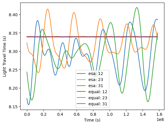
You can access various information on the orbits with the methods that begin with get. You can get light travel times, spacecraft positions, or link normal vectors. These functions require a linear interpolation setup.
Link light travel times.
[14]:
t_vals = np.linspace(0.0, np.min([esa.t_base.max(), equal.t_base.max()]), 1000)
for orbits, name in zip([esa, equal], ["esa", "equal"]):
    for link in [12, 23, 31]:
        plt.plot(t_vals, orbits.get_light_travel_times(t_vals, link), label=f"{name}: {link}")
plt.legend()
plt.ylabel("Light Travel Time (s)")
plt.xlabel("Time (s)")
[14]:
Text(0.5, 0, 'Time (s)')
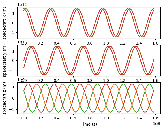
Spacecraft positions
[15]:
t_vals = np.linspace(0.0, np.min([esa.t_base.max(), equal.t_base.max()]), 1000)
fig, ax = plt.subplots(3, 1)
for orbits, name in zip([esa, equal], ["esa", "equal"]):
    for sc in [1, 2, 3]:
        pos = orbits.get_pos(t_vals, sc)
        for i in range(3):
            ax[i].plot(t_vals, pos[:, i], color=f"C{sc}", label=f"{name}: {link}")
ax[0].set_ylabel("spacecraft x (m)")
ax[1].set_ylabel("spacecraft y (m)")
ax[2].set_ylabel("spacecraft z (m)")
ax[2].set_xlabel("Time (s)")
[15]:
Text(0.5, 0, 'Time (s)')
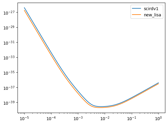
Defining a LISAModel
A LISAModel is a combination of sensitivity information and orbits. For the sensitivity, we define a two parameter model based on the OMS noise and acceleration noise.
[16]:
oms_noise_term = (13.0e-12) ** 2
acceleration_noise_term = (2.0e-15) ** 2
equal = EqualArmlengthOrbits()
new_lisa = LISAModel(oms_noise_term, acceleration_noise_term, equal, "new_lisa")
[17]:
# example stock model
get_available_default_lisa_models()
[17]:
[LISAModel(Soms_d=2.25e-22, Sa_a=9e-30, orbits=<lisatools.detector.DefaultOrbits object at 0x7f153a79ee70>, name='scirdv1'),
 LISAModel(Soms_d=9.999999999999999e-23, Sa_a=9e-30, orbits=<lisatools.detector.DefaultOrbits object at 0x7f153cfe7530>, name='proposal'),
 LISAModel(Soms_d=9.999999999999999e-23, Sa_a=5.76e-30, orbits=<lisatools.detector.DefaultOrbits object at 0x7f153d254080>, name='mrdv1'),
 LISAModel(Soms_d=6.241e-23, Sa_a=5.76e-30, orbits=<lisatools.detector.DefaultOrbits object at 0x7f153a79f680>, name='sangria'),
 ExtendedLISAModel(isi_oms_level=6.35e-12, rfi_oms_level=3.32e-12, tmi_oms_level=1.42e-12, tm_noise_level=2.4e-15, rfi_backlink_noise_level=3e-12, tmi_backlink_noise_level=3e-12, orbits=<lisatools.detector.DefaultOrbits object at 0x7f153a79f4d0>, name='sangria_v2')]
[18]:
f = np.logspace(-5, 0, 10000)

for model in [scirdv1, new_lisa]:
    Sn = get_sensitivity(f, sens_fn="LISASens", model=model)
    plt.loglog(f, Sn, label=model.name)
plt.legend()
[18]:
<matplotlib.legend.Legend at 0x7f1537559ca0>
Defining an ExtendedLISAModel
An ExtendedLISAModel is similar to the LISA Model. It has 6 noise components instead of 2:
Reference interferometer readout noise level
Test-mass interferometer readout noise level
Interspacecraft interferometer readout noise level
Reference interferometer backlink noise level
Test-mass interferometer backlink noise level
Test-mass acceleration noise level
[19]:
from lisatools.detector import ExtendedLISAModel, ExtendedLISAModelSettings
help(ExtendedLISAModel)
Help on class ExtendedLISAModel in module lisatools.detector:

class ExtendedLISAModel(ExtendedLISAModelSettings, abc.ABC)
 |  ExtendedLISAModel(isi_oms_level: 'float', rfi_oms_level: 'float', tmi_oms_level: 'float', tm_noise_level: 'float', rfi_backlink_noise_level: 'float', tmi_backlink_noise_level: 'float', orbits: 'Orbits', name: 'str') -> None
 |
 |  Model for the LISA Constellation
 |
 |  This includes sensitivity information computed in
 |  :py:mod:`lisatools.sensitivity` and orbital information
 |  contained in an :class:`Orbits` class object.
 |
 |  This class is used to house high-level methods useful
 |  to various needed computations.
 |
 |  Method resolution order:
 |      ExtendedLISAModel
 |      ExtendedLISAModelSettings
 |      abc.ABC
 |      builtins.object
 |
 |  Methods defined here:
 |
 |  __str__(self) -> 'str'
 |      Return str(self).
 |
 |  acc_2_ffd(self, f: 'float | np.ndarray') -> 'float | np.ndarray'
 |
 |  disp_2_ffd(self, f: 'float | np.ndarray') -> 'float | np.ndarray'
 |
 |  lisanoises(self, f: 'float | np.ndarray', unit: 'Optional[str]' = 'relative_frequency', method: 'Optional[str]' = 'modern') -> 'CurrentNoises'
 |      Calculate both LISA noise terms based on input model.
 |      Args:
 |          f: Frequency array.
 |          unit: Either ``"relative_frequency"`` or ``"displacement"``.
 |      Returns:
 |          Tuple with acceleration term as first value and oms term as second value.
 |
 |  ----------------------------------------------------------------------
 |  Data and other attributes defined here:
 |
 |  __abstractmethods__ = frozenset()
 |
 |  __annotations__ = {}
 |
 |  ----------------------------------------------------------------------
 |  Methods inherited from ExtendedLISAModelSettings:
 |
 |  __eq__(self, other)
 |      Return self==value.
 |
 |  __init__(self, isi_oms_level: 'float', rfi_oms_level: 'float', tmi_oms_level: 'float', tm_noise_level: 'float', rfi_backlink_noise_level: 'float', tmi_backlink_noise_level: 'float', orbits: 'Orbits', name: 'str') -> None
 |      Initialize self.  See help(type(self)) for accurate signature.
 |
 |  __repr__(self)
 |      Return repr(self).
 |
 |  ----------------------------------------------------------------------
 |  Data descriptors inherited from ExtendedLISAModelSettings:
 |
 |  __dict__
 |      dictionary for instance variables
 |
 |  __weakref__
 |      list of weak references to the object
 |
 |  ----------------------------------------------------------------------
 |  Data and other attributes inherited from ExtendedLISAModelSettings:
 |
 |  __dataclass_fields__ = {'isi_oms_level': Field(name='isi_oms_level',ty...
 |
 |  __dataclass_params__ = _DataclassParams(init=True,repr=True,eq=True,or...
 |
 |  __hash__ = None
 |
 |  __match_args__ = ('isi_oms_level', 'rfi_oms_level', 'tmi_oms_level', '...
[20]:
isi_oms_level = 6.35e-12
rfi_oms_level = 3.32e-12
tmi_oms_level = 1.42e-12
tm_noise_level = 2.4e-15
rfi_backlink_level = 3.0E-12
tmi_backlink_level = 3.0E-12
extended = ExtendedLISAModel(isi_oms_level, rfi_oms_level, tmi_oms_level, tm_noise_level, rfi_backlink_level, tmi_backlink_level, equal, "extended")
[21]:
# example stock model
get_available_default_lisa_models()
[21]:
[LISAModel(Soms_d=2.25e-22, Sa_a=9e-30, orbits=<lisatools.detector.DefaultOrbits object at 0x7f153a79ee70>, name='scirdv1'),
 LISAModel(Soms_d=9.999999999999999e-23, Sa_a=9e-30, orbits=<lisatools.detector.DefaultOrbits object at 0x7f153cfe7530>, name='proposal'),
 LISAModel(Soms_d=9.999999999999999e-23, Sa_a=5.76e-30, orbits=<lisatools.detector.DefaultOrbits object at 0x7f153d254080>, name='mrdv1'),
 LISAModel(Soms_d=6.241e-23, Sa_a=5.76e-30, orbits=<lisatools.detector.DefaultOrbits object at 0x7f153a79f680>, name='sangria'),
 ExtendedLISAModel(isi_oms_level=6.35e-12, rfi_oms_level=3.32e-12, tmi_oms_level=1.42e-12, tm_noise_level=2.4e-15, rfi_backlink_noise_level=3e-12, tmi_backlink_noise_level=3e-12, orbits=<lisatools.detector.DefaultOrbits object at 0x7f153a79f4d0>, name='sangria_v2')]
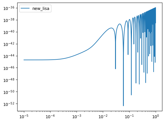
Plot the extended model.
[22]:
f = np.logspace(-5, 0, 10000)
Sn = get_sensitivity(f, sens_fn="X2TDISens", model=extended)
plt.loglog(f, Sn, label=model.name)
plt.legend()
[22]:
<matplotlib.legend.Legend at 0x7f1531ba9ca0>
Diagnostics
LISA Analysis Tools comes with a wide variety of diagnostic computations. These can be used in actual pipelines. However, they are slower, so these should mainly be used to check faster Likelihood methods.
To begin, we will define a basic sine wave as our waveform.
[23]:
def sine_waveform(A, f0, phi0, t_arr):
    return A * np.sin(2 * np.pi * f0 * t_arr + phi0)
Inner Product
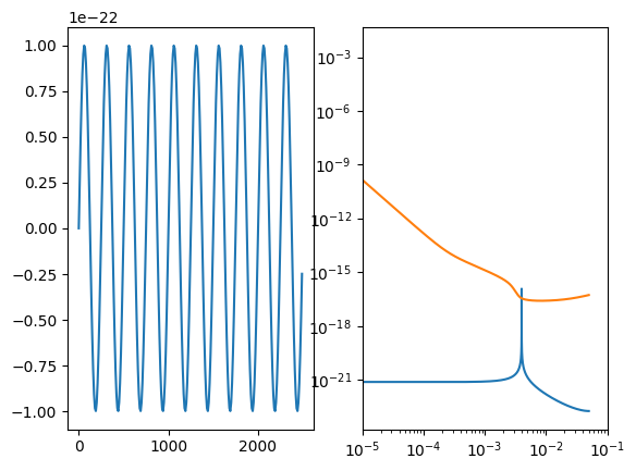
You can take the inner product between to waveforms. See the inner product documentation for keyword arguments and details.
[24]:
# create some fake signals first

A = 1e-22
f0 = 4e-3
phi0 = 0.2

dt = 10.0
t_arr = np.arange(0.0, YRSID_SI, dt)
df = 1 / (len(t_arr) * dt)
h1 = sine_waveform(A, f0, 0.0, t_arr)
h2 = sine_waveform(A, f0, phi0, t_arr)

fig, (ax1, ax2) = plt.subplots(1, 2)
ax1.plot(t_arr[:250], h1[:250])

freqs = np.fft.rfftfreq(len(h1), dt)
ax2.loglog(freqs, np.abs(np.fft.rfft(h1)))

ax2.loglog(freqs, (get_sensitivity(freqs, sens_fn="LISASens", model="sangria", stochastic_params=(YRSID_SI,)) / (4 * df)) ** (1/2))

val = inner_product(h1, h2, dt=dt, psd="LISASens", psd_kwargs=dict(model="sangria", stochastic_params=(YRSID_SI,)))
print(f"Inner product <h1|h2>: {val}")

complex_val = inner_product(h1, h2, dt=dt, psd="LISASens", psd_kwargs=dict(model="sangria", stochastic_params=(YRSID_SI,)), complex=True)
print(f"Complex inner product <h1|h2>: {complex_val}, phase maximized value: {np.abs(complex_val)}")

normalized_val = inner_product(h1, h2, dt=dt, psd="LISASens", psd_kwargs=dict(model="sangria", stochastic_params=(YRSID_SI,)), normalize=True)
print(f"Normalized inner product <h1|h2>: {normalized_val}")

ax2.set_xlim(1e-5,)
/opt/hostedtoolcache/Python/3.12.12/x64/lib/python3.12/site-packages/lisatools/detector.py:655: RuntimeWarning: divide by zero encountered in divide
  Sa_a = Sa_a_in * (1.0 + (0.4e-3 / frq) ** 2) * (1.0 + (frq / 8e-3) ** 4)
/opt/hostedtoolcache/Python/3.12.12/x64/lib/python3.12/site-packages/lisatools/detector.py:657: RuntimeWarning: divide by zero encountered in power
  Sa_d = Sa_a * (2.0 * np.pi * frq) ** (-4.0)
/opt/hostedtoolcache/Python/3.12.12/x64/lib/python3.12/site-packages/lisatools/detector.py:659: RuntimeWarning: invalid value encountered in multiply
  Sa_nu = Sa_d * (2.0 * np.pi * frq / C_SI) ** 2
/opt/hostedtoolcache/Python/3.12.12/x64/lib/python3.12/site-packages/lisatools/detector.py:664: RuntimeWarning: divide by zero encountered in divide
  Soms_d = Soms_d_in * (1.0 + (2.0e-3 / f) ** 4)
/opt/hostedtoolcache/Python/3.12.12/x64/lib/python3.12/site-packages/lisatools/detector.py:666: RuntimeWarning: invalid value encountered in multiply
  Soms_nu = Soms_d * (2.0 * np.pi * frq / C_SI) ** 2
/opt/hostedtoolcache/Python/3.12.12/x64/lib/python3.12/site-packages/lisatools/stochastic.py:178: RuntimeWarning: divide by zero encountered in power
  * (f ** (-7.0 / 3.0))
Inner product <h1|h2>: 1981.3392667268322
Complex inner product <h1|h2>: (1981.3392667268322+401.6384179983897j), phase maximized value: 2021.6376304090381
Normalized inner product <h1|h2>: 0.980066432814469
[24]:
(1e-05, np.float64(0.10206431774793984))
SNR
[25]:
opt_snr = snr(h1, dt=dt, psd="LISASens", psd_kwargs=dict(model="sangria", stochastic_params=(YRSID_SI,)))
print(f"Optimal SNR <h1|h1>^(1/2): {opt_snr}")

det_snr = snr(h1, data=h2, dt=dt, psd="LISASens", psd_kwargs=dict(model="sangria", stochastic_params=(YRSID_SI,)))
print(f"Detected SNR against data h1 <h1|h2> / <h1|h1>^(1/2): {det_snr}")
Optimal SNR <h1|h1>^(1/2): 44.96261510900949
Detected SNR against data h1 <h1|h2> / <h1|h1>^(1/2): 44.06637073762679
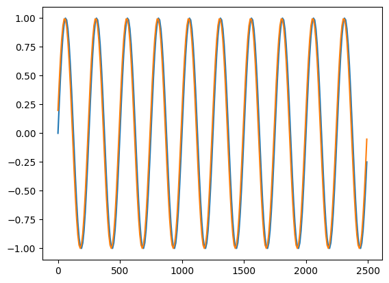
Perturbed Waveform
Get a waveform with a small perturbation to a parameter.
[26]:
# set quantities for below calculations
params = np.array([np.log(A), f0 * 1e3, phi0])
eps = 1e-9
index = 1

parameter_transforms = {
    "amp": np.exp,
    "f": lambda x: x / 1e3
}

input_basis = ["amp", "f", "phi0"]
output_basis = input_basis
transform_fn = TransformContainer(input_basis, output_basis, parameter_transforms=parameter_transforms)
[27]:
params = np.array([np.log(A), f0 * 1e3, phi0])
step = 1e-9
index = 1

parameter_transforms = {
    "amp": np.exp,
    "f": lambda x: x / 1e3
}

input_basis = ["amp", "f", "phi0"]
output_basis = input_basis
transform_fn = TransformContainer(input_basis, output_basis, parameter_transforms=parameter_transforms)

# will return 2D
dh = h_var_p_eps(
    step,
    sine_waveform,
    params,
    index,
    waveform_args=(t_arr,),
    parameter_transforms=transform_fn
)

plt.plot(t_arr[:250], h1[:250] / np.abs(h1[:250]).max())
plt.plot(t_arr[:250], dh[0, :250] / np.abs(dh[0, :250]).max())
[27]:
[<matplotlib.lines.Line2D at 0x7f1531ab4980>]
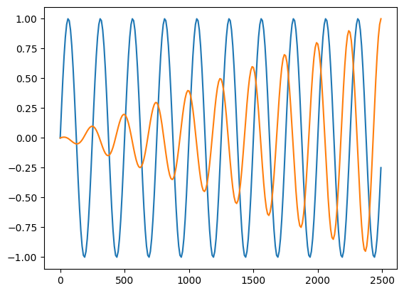
Derivative of Waveform
Compute the derivative of a waveform with respect to a parameter.
[28]:
dhdlam = dh_dlambda(
    eps,
    sine_waveform,
    params,
    index,
    waveform_args=(t_arr,),
    parameter_transforms=transform_fn
)

# TODO: check this?
plt.plot(t_arr[:250], h1[:250] / np.abs(h1[:250]).max())
plt.plot(t_arr[:250], dhdlam[0, :250] / np.abs(dhdlam[0, :250]).max())
[28]:
[<matplotlib.lines.Line2D at 0x7f1531975ca0>]
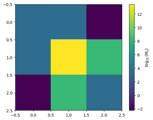
Information Matrix and Covariance
Information matrix and covariance matrices.
[29]:
params = np.array([np.log(A), f0 * 1e3, phi0])
eps = 1e-9

info_mat_args = (eps, sine_waveform, params)
info_mat_kwargs = dict(
    deriv_inds=None,
    inner_product_kwargs={
        "psd": "LISASens",
        "psd_kwargs": dict(model="sangria", stochastic_params=(YRSID_SI,)),
        "dt": dt,
    },
    return_derivs=False,
    waveform_args=(t_arr,),
    parameter_transforms=transform_fn,
)
im = info_matrix(*info_mat_args, **info_mat_kwargs)

cov = covariance(
    *info_mat_args,
    info_mat=None,
    diagonalize=False,
    return_info_mat=False,
    precision=True,
    **info_mat_kwargs,
)
print(cov)
mpmath module not installed. Defaulting to low precision...
[[ 4.94652789e-04 -1.34367850e-13  1.19037151e-08]
 [-1.34368053e-13  1.46157988e-13 -1.45604730e-08]
 [ 1.19037377e-08 -1.45604730e-08  1.95551222e-03]]
Visualizing your information matrix.
[30]:
plt.imshow(np.log10(im))
plt.colorbar(label=r"$\log_{10}(M_{ij})$")
[30]:
<matplotlib.colorbar.Colorbar at 0x7f1537577830>
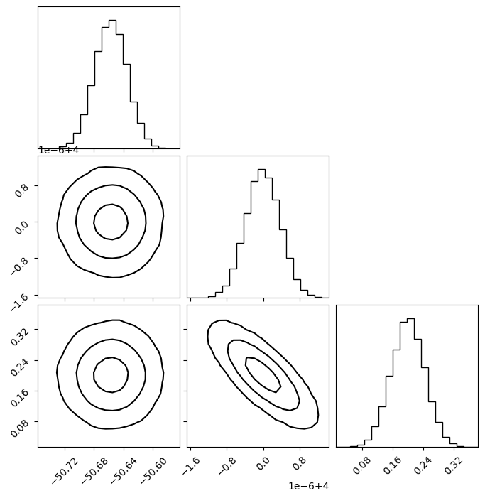
Plot Covariance in Corner Plot
You can plot a corner plot by generated samples from the covariance matrix.s
[31]:
plot_kwargs = dict(
    plot_density=False,
    plot_datapoints=False,  # fake in this case
    smooth=0.8,
    levels=1 - np.exp(-0.5 * np.array([1, 2, 3]) ** 2)  # 1, 2, 3 sigma
)

plot_covariance_corner(
    params,
    cov,
    **plot_kwargs
)
[31]:

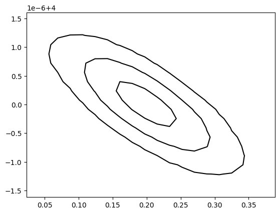
Make a single contour plot.
[32]:
fig, ax = plt.subplots(1,1)

plot_covariance_contour(
    params,
    cov,
    2,
    1,
    ax=ax,
    **plot_kwargs
)
[32]:
<Axes: >
Get Eigeninfo of a matrix (high-precision capability)
Get eigenvectors and eigenvalues of a matrix with high-precision capability.
[33]:
evals, evecs = get_eigeninfo(
    cov, high_precision=False
)
evals, evecs
[33]:
(array([4.94652788e-04, 1.95551222e-03, 3.77427245e-14]),
 array([[ 1.00000000e+00,  8.14843296e-06,  9.24576542e-11],
        [-3.17855070e-11, -7.44586141e-06,  1.00000000e+00],
        [-8.14844843e-06,  1.00000000e+00,  7.44586140e-06]]))
Scale to a given SNR
Scaled an injection signal to a given SNR in place.
[34]:
target_snr = 30.0

# with 0.0 for the phase here, h1/h1_scaled will have a nan at the beginning.
h1 = sine_waveform(A, f0, 0.2, t_arr)

h1_scaled = scale_to_snr(
    target_snr,
    h1,
    dt=dt,
    psd="LISASens",
    psd_kwargs=dict(model="sangria", stochastic_params=(YRSID_SI,))
)

print(h1 / h1_scaled)
[1.49875455 1.49875455 1.49875455 ... 1.49875455 1.49875455 1.49875455]
/opt/hostedtoolcache/Python/3.12.12/x64/lib/python3.12/site-packages/lisatools/detector.py:655: RuntimeWarning: divide by zero encountered in divide
  Sa_a = Sa_a_in * (1.0 + (0.4e-3 / frq) ** 2) * (1.0 + (frq / 8e-3) ** 4)
/opt/hostedtoolcache/Python/3.12.12/x64/lib/python3.12/site-packages/lisatools/detector.py:657: RuntimeWarning: divide by zero encountered in power
  Sa_d = Sa_a * (2.0 * np.pi * frq) ** (-4.0)
/opt/hostedtoolcache/Python/3.12.12/x64/lib/python3.12/site-packages/lisatools/detector.py:659: RuntimeWarning: invalid value encountered in multiply
  Sa_nu = Sa_d * (2.0 * np.pi * frq / C_SI) ** 2
/opt/hostedtoolcache/Python/3.12.12/x64/lib/python3.12/site-packages/lisatools/detector.py:664: RuntimeWarning: divide by zero encountered in divide
  Soms_d = Soms_d_in * (1.0 + (2.0e-3 / f) ** 4)
/opt/hostedtoolcache/Python/3.12.12/x64/lib/python3.12/site-packages/lisatools/detector.py:666: RuntimeWarning: invalid value encountered in multiply
  Soms_nu = Soms_d * (2.0 * np.pi * frq / C_SI) ** 2
/opt/hostedtoolcache/Python/3.12.12/x64/lib/python3.12/site-packages/lisatools/stochastic.py:178: RuntimeWarning: divide by zero encountered in power
  * (f ** (-7.0 / 3.0))
Bias estimate
Approximate waveform with a purposeful bias on the amplitude. Use the C-V bias estimate using our underlying covariance methods.
[35]:
def sine_waveform_approx(A, f0, phi0, t_arr):
    return A * 1.03 * np.sin(2 * np.pi * (f0 * 0.98) * t_arr + phi0)
[36]:
sys_err, bias = cutler_vallisneri_bias(
    sine_waveform,
    sine_waveform_approx,
    params,
    eps,
    parameter_transforms=transform_fn,
    inner_product_kwargs={
        "psd": "LISASens",
        "psd_kwargs": dict(model="sangria", stochastic_params=(YRSID_SI,)),
        "dt": dt,
    },
    waveform_true_args=(t_arr,),
    waveform_approx_args=(t_arr,),
)
print(sys_err, bias)
[2.02172681e+03 1.59046154e+04 1.94227074e-01] [ 1.00005281e+00 -7.75106971e-10 1.72300801e-04]
Data / Residual / Signal Container
This container is a holder for data, residuals, or templates. These communicate with other classes like the Sensitivity Matrix to streamline different analyses.
[37]:
from lisatools.datacontainer import DataResidualArray
[38]:
arr1 = sine_waveform(A, f0, phi0, t_arr)
arr2 = sine_waveform(A, f0, phi0 + np.pi / 2, t_arr)

data = DataResidualArray([arr1, arr2], dt=dt)
[39]:
data.loglog(char_strain=True)
[39]:
(<Figure size 640x480 with 2 Axes>, array([<Axes: >, <Axes: >], dtype=object))
Analysis Container
The AnalysisContainer brings together the SensitivityMatrix and the DataResidualArray to perform a variety of computations.
[40]:
from lisatools.analysiscontainer import AnalysisContainer
from lisatools.sensitivity import LISASens

sens_mat = SensitivityMatrix(data.f_arr, [LISASens, LISASens], stochastic_params=(YRSID_SI,))
analysis = AnalysisContainer(data, sens_mat)
[41]:
analysis.loglog()
/opt/hostedtoolcache/Python/3.12.12/x64/lib/python3.12/site-packages/lisatools/sensitivity.py:1249: RuntimeWarning: invalid value encountered in multiply
  plot_in = np.sqrt(self.frequency_arr * plot_in)
[41]:
(<Figure size 640x480 with 2 Axes>, array([<Axes: >, <Axes: >], dtype=object))
Direct computations on the residual contained in the DataResidualArrray.
[42]:
analysis.inner_product()
[42]:
4043.2899966962286
[43]:
analysis.likelihood()
[43]:
np.float64(287823726.7958254)
[44]:
analysis.likelihood(source_only=True)
[44]:
-2021.6449983481143
[45]:
analysis.likelihood(noise_only=True)
[45]:
np.float64(287825748.4408238)
[46]:
analysis.snr()
[46]:
63.58686968782335
Build a template and then compare it to the data.
[47]:
# build template
h_test = DataResidualArray([
    sine_waveform(A * 1.05, f0, phi0 + 0.002, t_arr),
    sine_waveform(A * 1.05, f0, phi0 + 0.002 + np.pi / 2., t_arr)
] , dt=dt)

print(f"Template Inner product: {analysis.template_inner_product(h_test)}") # , analysis.template_likelihood, analysis.template_snr
print(f"Template SNR: {analysis.template_snr(h_test)}") # , analysis.template_likelihood, analysis.template_snr
print(f"Template Likelihood: {analysis.template_likelihood(h_test)}") # , analysis.template_likelihood, analysis.template_snr
Template Inner product: 4245.446005624857
Template SNR: (np.float64(66.76621317221453), np.float64(63.586742514126044))
Template Likelihood: -5.062603402055174
Build a template generation model and add to the AnalysisContainer
This allows for inputing parameters and waveform settings directly to the AnalysisContainer for computations.
[48]:
def signal_model_sine(A, f0, phi0, t_arr):
    template = DataResidualArray([
        sine_waveform(A, f0, phi0, t_arr),
        sine_waveform(A, f0, phi0 + np.pi / 2., t_arr)
    ] , dt=dt)
    return template

analysis.signal_gen = signal_model_sine
[49]:
print(f"With parameters likelihood: {analysis.calculate_signal_likelihood(A, f0, phi0, t_arr, source_only=True)}")
print(f"With parameters snr: {analysis.calculate_signal_snr(A, f0, phi0, t_arr)}")
print(f"With parameters inner product: {analysis.calculate_signal_inner_product(A, f0, phi0, t_arr)}")

print("Adjust amplitude:")
print(f"With parameters likelihood: {analysis.calculate_signal_likelihood(A * 1.03, f0, phi0, t_arr, source_only=True)}")
print(f"With parameters snr: {analysis.calculate_signal_snr(A * 1.03, f0, phi0, t_arr)}")
print(f"With parameters inner product: {analysis.calculate_signal_inner_product(A * 1.03, f0, phi0, t_arr)}")
With parameters likelihood: -9.094947017729282e-13
With parameters snr: (np.float64(63.58686968782335), np.float64(63.586869687823345))
With parameters inner product: 4043.2899966962286
Adjust amplitude:
With parameters likelihood: -1.8194804985123483
With parameters snr: (np.float64(65.49447577845805), np.float64(63.58686968782337))
With parameters inner product: 4164.588696597116
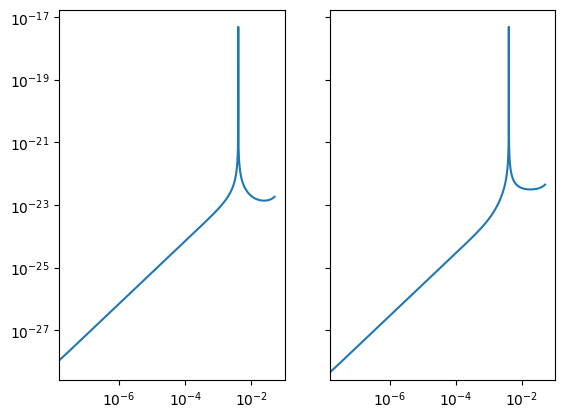
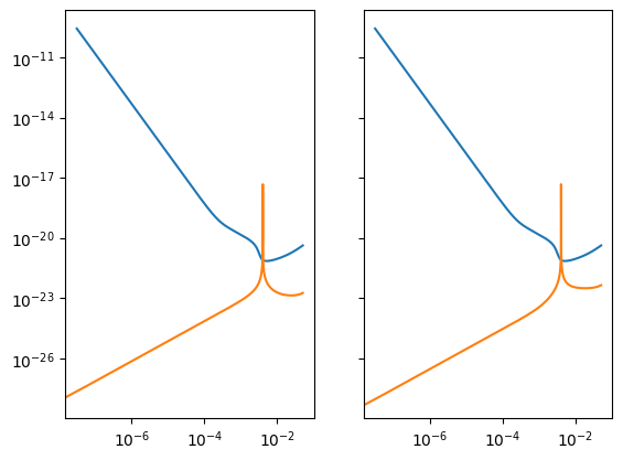
Comparing XYZ and AET
The XYZ TDI channels have correlated noise. In matrix form, you can imagine this as
.
For AET, this becomes diagonalized:
In the inner product equation, the multiplication of the template and noise is given as \((\mathbf{h}^T \mathbf{C}^{-1} \mathbf{h})\). In the XYZ basis, the full 3x3 matrix at each frequency must be inverted. In the AET basis, the inversion is equivalent to taking 1 over the sensitivity value themselves.
A good check is to verify that your inner product values are equivalent in both bases. To do this, you need real TDI templates. So, we will use GBGPU to put in one Galactic binary waveform.
[50]:
# setup a data stream
dt = 10.0
Tobs = YRSID_SI / 2.0
N = int(Tobs / dt)
Tobs = N * dt
t = np.arange(N) * dt

data_xyz = DataResidualArray(
    [
        np.zeros_like(t),
        np.zeros_like(t),
        np.zeros_like(t),
    ],
    dt=dt,
)

data_aet = DataResidualArray(
    [
        np.zeros_like(t),
        np.zeros_like(t),
        np.zeros_like(t),
    ],
    dt=dt,
)

# build waveforms
from gbgpu.gbgpu import GBGPU
gb = GBGPU()
gb.run_wave(
    1e-23, 0.003, 1e-17, 0.0, 0.4, 0.8, 0.9, 0.3, 0.5, T=Tobs, dt=dt, oversample=4
)

# inject waveforms
data_xyz[:, gb.start_inds[0] : gb.start_inds[0] + gb.A.shape[-1]] = (
    gb.XYZf[:]
)
data_aet[:, gb.start_inds[0] : gb.start_inds[0] + gb.A.shape[-1]] = (
    np.asarray(AET(*gb.XYZf[0]))
)

# set sensitivity matrices
sens_xyz = XYZ1SensitivityMatrix(data_xyz.f_arr, model="scirdv1")
sens_aet = AET1SensitivityMatrix(data_aet.f_arr, model="scirdv1")

ac_xyz = AnalysisContainer(data_xyz, sens_xyz)
ac_aet = AnalysisContainer(data_aet, sens_aet)

print(ac_xyz.inner_product(), ac_aet.inner_product())
print(ac_xyz.likelihood(source_only=True), ac_aet.likelihood(source_only=True))

# TODO: currently a small difference in noise-included likelihoodm
print(ac_xyz.likelihood(), ac_aet.likelihood())
19.13416533839461 19.13416533839472
-9.567082669197305 -9.56708266919736
216407643.55701742 216407890.27860746